Curvature Tensors

Consider the following figure, which depicts the parallel transport of vectors along a closed loop on a sphere:

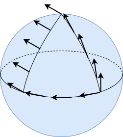
If the vector on the bottom right is parallel transported toward the north pole, then toward the equator, then along the equator, returning to its original point, the direction of the vector changes: it was originally pointing "northward", but now is pointing "westward". This change in direction is due to the curvature of the sphere.

However, when the same process is performed on a cylinder, the resultant vector is the same as the original vector, as in the following figure:

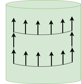
This is because a cylinder is an example of a "flat" manifold; it has no intrinsic curvature, although, when embedded in 3-dimensional space, it can be considered to have extrinsic curvature.

In fact, this observation can be used to define and measure curvature on arbitrary manifolds. The idea is as follows: parallel transport vectors along closed, "rectangular" loops, as in the following figure:

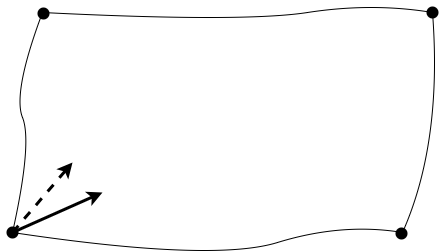
Measure the displacement vector as the difference between the original vector and the transported vector. Next, contract this rectangle, so that it becomes arbitrarily small. Define curvature as an appropriate limit involving the displacement vector.

To make this precise, we need the notion of a parametric family of curves, i.e. we need to be able to trace the outline of each rectangle using curves.

Definition (Parametric Family of Curves). A parametric family of curves is continuous map $\mathrm{\Gamma }:J\times I\to M$, where $I,J\subseteq \mathbb{R}$ are intervals and $M$ is a smooth manifold. The primary curves are the curves ${\mathrm{\Gamma }}_s:I\to M$, one for each $s\in J$, defined as ${\mathrm{\Gamma }}_s(t)=\mathrm{\Gamma }(s,t)$ for every $t\in I$. The transverse curves are the curves ${\mathrm{\Gamma }}^{(t)}:J\to M$, one for each $t\in I$, defined as ${\mathrm{\Gamma }}^{(t)}(s)=\mathrm{\Gamma }(s,t)$ for every $s\in J$.

A parametric family of curves thus represents a sort of "grid" of "horizontal" and "vertical" curves that can be overlayed on a manifold. They can be used to "trace" the "rectangles" described above.

Just as we can define vector fields along curves, we can likewise define vector fields along families of curves.

Definition (Vector Field along a Family of Curves). A vector field along a parametric family of curves $\mathrm{\Gamma }:J\times I\to M$ is a continuous map $V:J\times I\to TM$ such that $V(s,t)\in T_{\mathrm{\Gamma }(s,t)}M$ for all $(s,t)\in J\times I$.

We denote the velocity vectors of the primary curves as

$${\partial }_s\mathrm{\Gamma }(s,t)=({\mathrm{\Gamma }}_s{)}^{\prime }(t)\in T_{\mathrm{\Gamma }(s,t)}M$$

and we denote the velocity vectors of the transverse curves as

$${\partial }_t\mathrm{\Gamma }(s,t)=({\mathrm{\Gamma }}^{(t)}{)}^{\prime }(s)\in T_{\mathrm{\Gamma }(s,t)}M.$$

Thus, the velocity vectors are examples of vector fields along $\mathrm{\Gamma }$.

We likewise use the following notation:

• $$V_s:I\to TM,V_s(t)=V(s,t),$$
• $$V^{(t)}:J\to TM,V_t(s)=V(s,t).$$

Likewise, just as we can define the covariant derivative of a vector field along a curve, we can also define the covariant derivative of a vector field along a parametric family of curves using only a slightly modified definition.

Definition (Covariant Derivative along a Family of Curves). Given a family of curves $\mathrm{\Gamma }:J\times I\to M$, the primary covariant derivative of a vector field $V:J\times I\to TM$ along $\mathrm{\Gamma }$ is defined as

$$D_{t}V(s,t)=D_t{V}_s(t),$$

where $D_t{V}_s(t)$ is the covariant derivative along the primary curve ${\mathrm{\Gamma }}_s$, and the transverse covariant derivative of a $V$ along $\mathrm{\Gamma }$ is defined as

$$D_{s}V(s,t)=D_s{V}^{(t)}(s),$$

where $D_s{V}^{(t)}(s)$ is the covariant derivative along the transverse curve ${\mathrm{\Gamma }}^{(t)}$.

Thus, given smooth coordinates $(x^i)$ in a neighborhood of $\mathrm{\Gamma }(s,t)$, the coordinate expressions are as follows:

$$\begin{array}{rl}{D}_{t}V(s,t)& =D_t{V}_s(t)\\ & =D_t(V_s^i(t){\partial }_i{|}_{{\mathrm{\Gamma }}_s(t)})\\ & ={\dot{V}}_s^i(t){\partial }_i{|}_{{\mathrm{\Gamma }}_s(t)}+V_s^i(t)D_t{\partial }_i{|}_{{\mathrm{\Gamma }}_s(t)}\\ & =\frac{\partial V^i}{\partial t}(s,t){\partial }_i{|}_{\mathrm{\Gamma }(s,t)}+V^i(s,t)D_t{\partial }_i{|}_{\mathrm{\Gamma }(s,t)}.\end{array}$$

$$\begin{array}{rl}{D}_{s}V(s,t)& =D_s{V}^{(t)}(s)\\ & =D_s((V^{(t)}{)}^i{\partial }_i{|}_{{\mathrm{\Gamma }}^{(t)}(s)})\\ & =((V^{(t)}{)}^i{)}^{\prime }(s){\partial }_i{|}_{{\mathrm{\Gamma }}^{(t)}(s)}+(V^{(t)}{)}^i(s)D_s{\partial }_i{|}_{{\mathrm{\Gamma }}^{(t)}(s)}\\ & =\frac{\partial V^i}{\partial s}(s,t){\partial }_i{|}_{\mathrm{\Gamma }(s,t)}+V^i(s,t)D_s{\partial }_i{|}_{\mathrm{\Gamma }(s,t)}.\end{array}$$

Likewise, we can also define parallel transport for families of curves.

Definition (Parallel Transport along a Family of Curves). Given a Riemannian (or semi-Riemannian) manifold $M$ and a smooth family of curves $\mathrm{\Gamma }:I\times I\to M$ defined on an open interval $I\subseteq \mathbb{R}$ such that $0\in I$, the parallel transport along the primary curve ${\mathrm{\Gamma }}_s$ from time $t_1$ to time $t_2$ is defined as

$$P_{s_1,t_1}^{s_1,t_2}=P_{t_1,t_2}^{{\mathrm{\Gamma }}_{s_1}}:T_{\mathrm{\Gamma }(s_1,t_1)}M\to T_{\mathrm{\Gamma }(s_2,t_2)}M.$$

Likewise, the parallel transport along the transverse curve ${\mathrm{\Gamma }}^{(t)}$ from time $s_1$ to time $s_2$ is defined as

$$P_{s_1,t_1}^{s_2,t_1}=P_{s_1,s_2}^{{\mathrm{\Gamma }}^{(t_1)}}:T_{\mathrm{\Gamma }(s_1,t_1)}M\to T_{\mathrm{\Gamma }(s_2,t_1)}M.$$

We are now prepared to define the curvature measure proposed in the introduction.

Definition (Displacement). Given a Riemannian (or semi-Riemannian) manifold $M$ and a smooth family of curves $\mathrm{\Gamma }:I\times I\to M$ defined on an open interval $I\subseteq \mathbb{R}$ such that $0\in I$, the displacement along $\mathrm{\Gamma }$ at the point $p=\mathrm{\Gamma }(0,0)$ is defined for each $z\in T_{p}M$ as follows:

$${\mathcal{D}}_p(z)=\underset{\delta ,\epsilon \to 0}{lim}\frac{P_{\delta ,0}^{0,0}\circ P_{\delta ,\epsilon }^{\delta ,0}\circ P_{0,\epsilon }^{\delta ,\epsilon }\circ P_{0,0}^{0,\epsilon }(z)-z}{\delta \epsilon }.$$

The displacement is the limiting ratio of the displacement vector resulting from parallel transport around the "rectangular" loop and the area $\delta \epsilon$ of the rectangular interval $(0,\delta )\times (0,\epsilon )$ in the domain of $\mathrm{\Gamma }$.

The limit $\underset{x,y\to a}{lim}f(x,y)=L$ is interpreted as follows: for all $\epsilon >0$, there exists a $\delta >0$ such that $\Vert f(x,y)-L\Vert <\epsilon$ whenever both $\Vert x-a\Vert <\delta$ and $\Vert y-a\Vert <\delta$. This is equivalent to $\underset{x\to a}{lim}\underset{y\to a}{lim}f(x,y)$.

This process is depicted in the following figure:

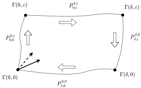
Let $Z$ denote the vector field along $\mathrm{\Gamma }$ defined by first parallel transporting the tangent vector $Z(0,0)=z$ "vertically" (according to the figure) along the primary curve ${\mathrm{\Gamma }}_0$ and then, for each $t$, parallel transporting "horizontally" (according to the figure) along the transverse curve ${\mathrm{\Gamma }}^{(t)}$. Then, $Z$ represents the process of transporting a vector $z$ around the closed, rectangular loop as depicted in the figure. $Z$ can thus be defined as follows:

$$Z(s,t)=P_{0,t}^{s,t}(P_{0,0}^{0,t}(z)).$$

This process is analogous to a derivative, and indeed bears a resemblance to the formula for the covariant derivative of a vector field $V$ along a curve $\gamma$ in terms of parallel transport:

$$D_{t}V(t_0)=\underset{t_1\to 0}{lim}\frac{P_{t,0}^{\gamma }V(t_0+t_1)-V(t_0)}{t_1}.$$

This formula then implies that

$$D_s{D}_{t}Z(0,0)=\underset{\delta \to 0}{lim}\frac{P_{\delta ,0}^{0,0}(D_{t}Z(\delta ,0))-D_{t}Z(0,0)}{\delta }.$$

Furthermore, the same formula implies that

$$D_{t}Z(\delta ,0)=\underset{\epsilon \to 0}{lim}\frac{P_{\delta ,\epsilon }^{\delta ,0}(Z(\delta ,\epsilon ))-Z(\delta ,0)}{\epsilon }$$

and

$$D_{t}Z(0,0)=\underset{\epsilon \to 0}{lim}\frac{P_{0,\epsilon }^{0,0}(Z(0,\epsilon ))-Z(0,0)}{\epsilon }.$$

Now, recall that limits in finite-dimensional normed vector spaces are computed component-wise, meaning that $\underset{h\to a}{lim}f(h)=(\underset{h\to a}{lim}{f}^j(h))\cdot e_j$ for any basis $(e_j$). It thus follows that, for any linear map $A:V\to W$ between finite-dimensional normed vector spaces $V$ and $W$ and any basis $(e_j)$ for $V$,

$$\begin{array}{rl}A(\underset{h\to a}{lim}f(h))& =A((\underset{h\to a}{lim}{f}^j(h))\cdot e_j)\\ & =(\underset{h\to a}{lim}{f}^j(h))\cdot A(e_j)\\ & =\underset{h\to a}{lim}(f^j(h)\cdot A(e_j))\\ & =\underset{h\to a}{lim}A(f^j(h)\cdot e_j)\\ & =\underset{h\to a}{lim}A(f(h)).\end{array}$$

Thus, limits "commute" with the application of linear maps. Since parallel transport is a linear map, it follows that

$$\begin{array}{rl}{P}_{\delta ,0}^{0,0}(D_{t}Z(\delta ,0))& =P_{\delta ,0}^{0,0}\left(\underset{\epsilon \to 0}{lim}\frac{P_{\delta ,\epsilon }^{\delta ,0}(Z(\delta ,\epsilon ))-Z(\delta ,0)}{\epsilon }\right)\\ & =\underset{\epsilon \to 0}{lim}{P}_{\delta ,0}^{0,0}\left(\frac{P_{\delta ,\epsilon }^{\delta ,0}(Z(\delta ,\epsilon ))-Z(\delta ,0)}{\epsilon }\right)\\ & =\underset{\epsilon \to 0}{lim}\frac{P_{\delta ,0}^{0,0}(P_{\delta ,\epsilon }^{\delta ,0}(Z(\delta ,\epsilon )))-P_{\delta ,0}^{0,0}(Z(\delta ,0))}{\epsilon }.\end{array}$$

Then, substituting, we obtain

$$\begin{array}{rl}{D}_s{D}_{t}Z(0,0)& =\underset{\delta \to 0}{lim}\frac{\left[\underset{\epsilon \to 0}{lim}\frac{P_{\delta ,0}^{0,0}(P_{\delta ,\epsilon }^{\delta ,0}(Z(\delta ,\epsilon )))-P_{\delta ,0}^{0,0}(Z(\delta ,0))}{\epsilon }\right]-\left[\underset{\epsilon \to 0}{lim}\frac{P_{0,\epsilon }^{0,0}(Z(0,\epsilon ))-Z(0,0)}{\epsilon }\right]}{\delta }\\ & =\underset{\delta \to 0}{lim}\frac{\underset{\epsilon \to 0}{lim}[\frac{P_{\delta ,0}^{0,0}(P_{\delta ,\epsilon }^{\delta ,0}(Z(\delta ,\epsilon )))-P_{\delta ,0}^{0,0}(Z(\delta ,0))}{\epsilon }-\frac{P_{0,\epsilon }^{0,0}(Z(0,\epsilon ))-Z(0,0)}{\epsilon }]}{\delta }\\ & =\underset{\delta \to 0}{lim}\underset{\epsilon \to 0}{lim}\frac{[\frac{P_{\delta ,0}^{0,0}(P_{\delta ,\epsilon }^{\delta ,0}(Z(\delta ,\epsilon )))-P_{\delta ,0}^{0,0}(Z(\delta ,0))}{\epsilon }-\frac{P_{0,\epsilon }^{0,0}(Z(0,\epsilon ))-Z(0,0)}{\epsilon }]}{\delta }\\ & =\underset{\delta ,\epsilon \to 0}{lim}\frac{P_{\delta ,0}^{0,0}(P_{\delta ,\epsilon }^{\delta ,0}(Z(\delta ,\epsilon )))-P_{\delta ,0}^{0,0}(Z(\delta ,0))-P_{0,\epsilon }^{0,0}(Z(0,\epsilon ))+Z(0,0)}{\delta \epsilon }.\end{array}$$

Next, recall that the parallel transport map is a linear isomorphism, whose inverse is parallel transport along the inverse curve (i.e. curve going "in the opposite direction" with the upper and lower indices swapped). Also note that $Z$ is parallel along ${\mathrm{\Gamma }}_0$ and along ${\mathrm{\Gamma }}^{(t)}$ for every $t$ by construction, and hence the result of parallel transport along such curves to an index is the same as the value of $Z$ at the respective index. It then follows that

$$\begin{array}{rl}z& =Z(0,0)\\ & =P_{0,\epsilon }^{0,0}(P_{0,0}^{0,\epsilon }(Z(0,0)))\\ & =P_{0,\epsilon }^{0,0}(Z(0,\epsilon )),\end{array}$$

and likewise

$$\begin{array}{rl}z& =Z(0,0)\\ & =P_{0,\epsilon }^{\delta ,\epsilon }(P_{\delta ,\epsilon }^{0,\epsilon }(Z(0,0)))\\ & =P_{0,\epsilon }^{\delta ,\epsilon }(Z(0,\epsilon )).\end{array}$$

It also follows that

$$\begin{array}{rl}Z(\delta ,\epsilon )& =P_{0,\epsilon }^{\delta ,\epsilon }(Z(0,\epsilon ))\\ & =P_{0,\epsilon }^{\delta ,\epsilon }(P_{0,0}^{0,\epsilon }(z)).\end{array}$$

If we substitute this into the limit obtained previously, we obtain

$$D_s{D}_{t}Z(0,0)=\underset{\delta ,\epsilon \to 0}{lim}\frac{P_{\delta ,0}^{0,0}\circ P_{\delta ,\epsilon }^{\delta ,0}\circ P_{0,\epsilon }^{\delta ,\epsilon }\circ P_{0,0}^{0,\epsilon }(z)-z}{\delta \epsilon }.$$

Thus, we have obtained an equivalent expression for displacement:

$${\mathcal{D}}_p(z)=D_s{D}_{t}Z(0,0),$$

where $\mathrm{\Gamma }$ is an appropriately defined family of curves, $Z$ is an appropriately defined vector field along $\mathrm{\Gamma }$, and $Z(0,0)=z$.

Definition (Displacement [Alternative]). Given a Riemannian (or semi-Riemannian) manifold $M$ and a smooth family of curves $\mathrm{\Gamma }:I\times I\to M$ defined on an open interval $I\subseteq \mathbb{R}$ such that $0\in I$, the displacement along $\mathrm{\Gamma }$ at the point $p=\mathrm{\Gamma }(0,0)$ is defined for every tangent vector $z\in T_{p}M$ as

$${\mathcal{D}}_p(z)=D_s{D}_{t}Z(0,0),$$

where $Z$ is the vector field along $\mathrm{\Gamma }$ defined as

$$Z(s,t)=P_{0,t}^{s,t}(P_{0,0}^{0,t}(z)).$$

Although this is a useful and intuitive characterization of curvature, it is not yet complete since it is restricted to vector fields along families of curves. Instead, we seek a characterization of curvature which is applicable to arbitrary vector fields. The displacement operation indicates that curvature is somehow related to second covariant derivatives.

It is often instructive to consider the special case of the Euclidean connection $\overline{\mathrm{\nabla }}$. Recall that the Euclidean connection can be expressed in terms of smooth coordinates as

$${\overline{\mathrm{\nabla }}}_{X}Y=X(Y^i){\partial }_i.$$

We then compute the following in smooth coordinates (noting that ${\overline{\mathrm{\nabla }}}_X{\partial }_i=0$ for any $X$ in the Euclidean connnection):

$$\begin{array}{rl}{\overline{\mathrm{\nabla }}}_X{\overline{\mathrm{\nabla }}}_{Y}Z& ={\overline{\mathrm{\nabla }}}_X(Y(Z^i){\partial }_i)\\ & =Y(Z^i){\overline{\mathrm{\nabla }}}_X{\partial }_i+X(Y(Z^i)){\partial }_i& \text{(Product rule)}\\ & =X(Y(Z^i)){\partial }_i.\end{array}$$

Likewise, transposing $X$ and $Y$, it follows that

$${\overline{\mathrm{\nabla }}}_Y{\overline{\mathrm{\nabla }}}_{X}Z=Y(X(Z^i)){\partial }_i.$$

Again, it also follows that

$$\begin{array}{rl}{\overline{\mathrm{\nabla }}}_{[X,Y]}Z& =[X,Y](Z^i){\partial }_i\\ & =(XY-YX)(Z^i){\partial }_i\\ & =X(Y(Z^i)){\partial }_i-Y(X(Z^i)){\partial }_i\\ & ={\overline{\mathrm{\nabla }}}_X{\overline{\mathrm{\nabla }}}_{Y}Z-{\overline{\mathrm{\nabla }}}_Y{\overline{\mathrm{\nabla }}}_{X}Z.\end{array}$$

Thus, for the Euclidean connection,

$${\overline{\mathrm{\nabla }}}_X{\overline{\mathrm{\nabla }}}_{Y}Z-{\overline{\mathrm{\nabla }}}_Y{\overline{\mathrm{\nabla }}}_{X}Z-{\overline{\mathrm{\nabla }}}_{[X,Y]}Z=0.$$

Therefore, for the Euclidean connection, it is not sufficient to consider ${\overline{\mathrm{\nabla }}}_X{\overline{\mathrm{\nabla }}}_{Y}Z$ alone, but the additional terms in the expression above must also be considered, and, in particular, they obey the equation above.

We therefore generalize this formula and propose the following characterization of curvature for the Levi-Civita connection on arbitrary Riemannian (or semi-Riemannian) manifolds.

Definition (Riemann Curvature Endomorphism). For any Riemannian (or semi-Riemannian) manifold $M$ and smooth vector fields $X$ and $Y$ on $M$, the (Riemann) curvature endomorphism determined by $X$ and $Y$ is the map $R(X,Y):\mathfrak{X}(M)\to \mathfrak{X}(M)$, where $R:\mathfrak{X}(M)\times \mathfrak{X}(M)\times \mathfrak{X}(M)\to \mathfrak{X}(M)$ defined for all $Z\in \mathfrak{X}(M)$ as

$$R(X,Y)Z={\mathrm{\nabla }}_X{\mathrm{\nabla }}_{Y}Z-{\mathrm{\nabla }}_Y{\mathrm{\nabla }}_{X}Z-{\mathrm{\nabla }}_{[X,Y]}Z.$$

Thus, for the Euclidean connection, $R(X,Y)Z=0$ for all vector fields $X$,$Y$, and $Z$.

The following theorem holds (but its proof would require a detour, so it is omitted):

Theorem. A Riemannian (or semi-Riemannian) manifold is flat if and only if its curvature tensor vanishes identically.

Thus, the relation above holds for all flat manifolds (i.e. those locally isometric to Euclidean space). This verifies that the curvature endomorphism characterizes flatness, and likewise provides a concrete measure of the deviation from flatness for non-flat manifolds.

Next, we want to confirm that the Riemann curvature endomorphism is multilinear over $C^{\mathrm{\infty }}(M)$, which will allows us to derive a corresponding tensor field from this endomorphism.

First, note that

$$\begin{array}{rl}R(fX,Y)Z& ={\mathrm{\nabla }}_{fX}{\mathrm{\nabla }}_{Y}Z-{\mathrm{\nabla }}_Y{\mathrm{\nabla }}_{fX}Z-{\mathrm{\nabla }}_{[fX,Y]}Z\\ & =f{\mathrm{\nabla }}_X{\mathrm{\nabla }}_{Y}Z-{\mathrm{\nabla }}_Y(f{\mathrm{\nabla }}_{X}Z)-{\mathrm{\nabla }}_{(fXY-Y(fX))}Z\\ & =f{\mathrm{\nabla }}_X{\mathrm{\nabla }}_{Y}Z-f{\mathrm{\nabla }}_Y{\mathrm{\nabla }}_{X}Z-Yf{\mathrm{\nabla }}_{X}Z-{\mathrm{\nabla }}_{(fXY-fYX-YfX)}Z\\ & =f{\mathrm{\nabla }}_X{\mathrm{\nabla }}_{Y}Z-f{\mathrm{\nabla }}_Y{\mathrm{\nabla }}_{X}Z-Yf{\mathrm{\nabla }}_{X}Z-{\mathrm{\nabla }}_{(f[X,Y]-YfX)}Z\\ & =f{\mathrm{\nabla }}_X{\mathrm{\nabla }}_{Y}Z-f{\mathrm{\nabla }}_Y{\mathrm{\nabla }}_{X}Z-Yf{\mathrm{\nabla }}_{X}Z-f{\mathrm{\nabla }}_{[X,Y]}Z+Yf{\mathrm{\nabla }}_{X}Z\\ & =f{\mathrm{\nabla }}_X{\mathrm{\nabla }}_{Y}Z-f{\mathrm{\nabla }}_Y{\mathrm{\nabla }}_{X}Z-f{\mathrm{\nabla }}_{[X,Y]}Z\\ & =fR(X,Y)Z.\end{array}$$

A similar calculation shows that $R(X,fY)=fR(X,Y)Z$. Finally, note that

$$\begin{array}{rl}R(X,Y)(fZ)& ={\mathrm{\nabla }}_X{\mathrm{\nabla }}_Y(fZ)-{\mathrm{\nabla }}_Y{\mathrm{\nabla }}_X(fZ)-{\mathrm{\nabla }}_{[X,Y]}(fZ)\\ & ={\mathrm{\nabla }}_X(f{\mathrm{\nabla }}_{Y}Z+YfZ)-{\mathrm{\nabla }}_Y(f{\mathrm{\nabla }}_{X}Z+XfZ)-(f{\mathrm{\nabla }}_{[X,Y]}Z+[X,Y]fZ)\\ & ={\mathrm{\nabla }}_X(f{\mathrm{\nabla }}_{Y}Z)+{\mathrm{\nabla }}_X(YfZ)-{\mathrm{\nabla }}_Y(f{\mathrm{\nabla }}_{X}Z)-{\mathrm{\nabla }}_Y(XfZ)-f{\mathrm{\nabla }}_{[X,Y]}Z-[X,Y]fZ\\ & =(f{\mathrm{\nabla }}_X{\mathrm{\nabla }}_{Y}Z+Xf{\mathrm{\nabla }}_{Y}Z)+(Yf{\mathrm{\nabla }}_{X}Z+XYfZ)-(f{\mathrm{\nabla }}_Y{\mathrm{\nabla }}_{X}Z+Yf{\mathrm{\nabla }}_{X}Z)-(Xf{\mathrm{\nabla }}_{Y}Z+YXfZ)-f{\mathrm{\nabla }}_{[X,Y]}Z-(XYfZ-YXfZ)\\ & =f{\mathrm{\nabla }}_X{\mathrm{\nabla }}_{Y}Z-f{\mathrm{\nabla }}_Y{\mathrm{\nabla }}_{X}Z-f{\mathrm{\nabla }}_{[X,Y]}Z\\ & =fR(X,Y)Z.\end{array}$$

Tensors and Multilinear Maps

Tensor fields of type $(k+1,l)$ can be characterized by maps that are multilinear over $C^{\mathrm{\infty }}(M)$, either with signature

$$\underset{k+1\text{times}}{\underbrace{{\mathfrak{X}}^{\ast }(M)\times \cdots \times {\mathfrak{X}}^{\ast }(M)}}\times \underset{l\text{times}}{\underbrace{\mathfrak{X}(M)\cdots \times \mathfrak{X}(M)}}\to C^{\mathrm{\infty }}(M)$$

or with signature

$$\underset{k\text{times}}{\underbrace{{\mathfrak{X}}^{\ast }(M)\times \cdots \times {\mathfrak{X}}^{\ast }(M)}}\times \underset{l\text{times}}{\underbrace{\mathfrak{X}(M)\cdots \times \mathfrak{X}(M)}}\to \mathfrak{X}(M).$$

In this section we will review these results, which are crucial for formulating a curvature tensor based on the curvature endomorphism.

Linear Maps

For any vector spaces $V$ and $W$,

$$[V,W]\cong L(W^{\ast },V;\mathbb{R}),$$

where $[V,W]$ denotes the vector space of linear maps with signature $V\to W$ and $L(W^{\ast },V;\mathbb{R})$ denotes the vector space of multilinear maps with signature $W^{\ast }\times V\to \mathbb{R}$.

This isomorphism is witnessed by the following map:

$$\phi (A)(\omega ,v)=\omega (Av).$$

This is indeed an isomorphism, since it has a trivial kernel. Given a basis $(E_i^W)$ for $W$ with corresponding dual basis $({\epsilon }_W^j)$, the inverse mapping can be defined explicitly:

$${\phi }^{-1}(L)(v)=L({\epsilon }_W^i,v)\cdot E_i^W,$$

We then compute

$$\begin{array}{rl}\phi ({\phi }^{-1}(L))(\omega ,v)& =\omega (L({\epsilon }_W^i,v)\cdot E_i^W)\\ & =L({\epsilon }_W^i,v)\cdot \omega (E_i^W)\\ & ={\omega }^i\cdot L({\epsilon }_W^i,v)\\ & =L({\omega }^i\cdot {\epsilon }_W^i,v)\\ & =L(\omega ,v).\end{array}$$

Likewise, we also compute

$$\begin{array}{rl}{\phi }^{-1}(\phi (A))(v)& ={\epsilon }_W^i(Av)\cdot E_i^W\\ & =[Av{]}^i\cdot E_i^W\\ & =Av.\end{array}$$

If ${\phi }^{-1}(L)=A$, then it follows that

$$\begin{array}{rl}A(E_j^V)& ={\phi }^{-1}(L)(E_j^V)\\ & =L({\epsilon }_W^i,E_j^V)\cdot E_i^W\\ & =L_j^i\cdot E_i^W,\end{array}$$

where $L_j^i$ are the components of the tensor, and likewise if $\phi (A)=L$, then it follows that

$$\begin{array}{rl}{L}_j^i& =L({\epsilon }_W^i,E_j^V)\\ & =\phi (A)({\epsilon }_W^i,E_j^V)\\ & ={\epsilon }_W^i(A(E_j^V))\\ & =[A(E_j^V){]}^i.\end{array}$$

Thus, if only $A$ is known, the tensor components $L_j^i$ can be computed in this manner.

Multilinear Maps

Moreover, for any vector spaces $V_1,\dots ,V_k$ and $W$,

$$L(V_1,\dots ,V_k;W)\cong L(W^{\ast },V_1,\dots ,V_k;\mathbb{R}).$$

This isomorphism is witnessed by the following map:

$$\phi (A)(\omega ,v_1,\dots ,v_k)=\omega (A(v_1,\dots ,v_k)).$$

This is indeed an isomorphism, since it has a trivial kernel. Given a basis $(E_i^W)$ for $W$ with corresponding dual basis $({\epsilon }_W^i)$, the inverse mapping can be defined explicitly:

$${\phi }^{-1}(L)(v_1,\dots ,v_k)=L({\epsilon }_W^i,v_1,\dots ,v_k)\cdot E_i^W.$$

Multilinear Maps on a Vector Space

This can be restricted to multilinear maps "on" a vector space $V$, i.e. either covariant maps

$$L(\underset{k\text{times}}{\underbrace{V,\dots ,V}};V)\cong L(V^{\ast },\underset{k\text{times}}{\underbrace{V,\dots ,V}};\mathbb{R})$$

as witnessed by the map

$$\phi (A)(\omega ,v_1,\dots ,v_k)=\omega (A(v_1,\dots ,v_k)),$$

or contravariant maps

$$L(\underset{k\text{times}}{\underbrace{V^{\ast },\dots ,V^{\ast }}};V)\cong L(\underset{k+1\text{times}}{\underbrace{V^{\ast },\dots ,V^{\ast }}};\mathbb{R})$$

as witnessed by the map

$$\phi (A)({\omega }^1,\dots ,{\omega }^{k+1})={\omega }^{k+1}(A({\omega }^1,\dots ,{\omega }^k)),$$

or maps of mixed variance

$$L(\underset{k\text{times}}{\underbrace{V^{\ast },\dots ,V^{\ast }}},\underset{l\text{times}}{\underbrace{V,\dots ,V}};V)\cong L(\underset{k+1\text{times}}{\underbrace{V^{\ast },\dots ,V^{\ast }}},\underset{l\text{times}}{\underbrace{V,\dots ,V}};\mathbb{R})$$

as witnessed by the map

$$\phi (A)({\omega }^1,\dots ,{\omega }^{k+1},v_1,\dots ,v_l)={\omega }^{k+1}(A({\omega }^1,\dots ,{\omega }^k,v_1,\dots ,v_l)).$$

This is indeed an isomorphism, since it has a trivial kernel. Given a basis $(E_i^W)$ for $W$ with corresponding dual basis $({\epsilon }_W^i)$, the inverse mapping can be defined explicitly:

$${\phi }^{-1}(L)({\omega }^1,\dots ,{\omega }^k,v_1,\dots ,v_l)=L({\omega }^1,\dots ,{\omega }^k,{\epsilon }_W^{i_{k+1}},v_1,\dots ,v_l)\cdot E_{i_{k+1}}^W.$$

If ${\phi }^{-1}(L)=A$, then it follows that

$$\begin{array}{rl}A({\epsilon }_W^{i_1},\dots ,{\epsilon }_W^{i_k},E_{j_1},\dots ,E_{j_l})& ={\phi }^{-1}(L)({\epsilon }_W^{i_1},\dots ,{\epsilon }_W^{i_k},E_{j_1},\dots ,E_{j_l})\\ & =L({\epsilon }_W^{i_1},\dots ,{\epsilon }_W^{i_{k+1}},E_{j_1},\dots ,E_{j_l})\cdot E_{i_{k+1}}^W\\ & =L_{j_1,\dots ,j_l}^{i_1,\dots ,i_{k+1}}\cdot E_{i_{k+1}}^W,\end{array}$$

and likewise if $\phi (A)=L$, then it follows that

$$\begin{array}{rl}{L}_{j_1,\dots ,j_l}^{i_1,\dots ,i_{k+1}}& =L({\epsilon }_W^{i_1},\dots ,{\epsilon }_W^{i_{k+1}},E_{j_1},\dots ,E_{j_l})\\ & =\phi (A)({\epsilon }_W^{i_1},\dots ,{\epsilon }_W^{i_{k+1}},E_{j_1},\dots ,E_{j_l})\\ & ={\epsilon }_W^{i_{k+1}}(A({\epsilon }_W^{i_1},\dots ,{\epsilon }_W^{i_k},E_{j_1},\dots ,E_{j_l}))\cdot E_{i_{k+1}}^W\\ & =[A({\epsilon }_W^{i_1},\dots ,{\epsilon }_W^{i_k},E_{j_1},\dots ,E_{j_l}){]}^{i_{k+1}}\cdot E_{i_{k+1}}^W.\end{array}$$

Thus, if only $A$ is known, the tensor components $L_{j_1,\dots ,j_k}^{i_1,\dots ,i_{k+1}}$ can be computed in this manner.

The Characterization Lemma

Given any tensor field $F:M\to T^{(k,l)}TM$, smooth covector fields ${\omega }^1,\dots ,{\omega }^k$, and smooth vector fields $X_1,\dots ,X_l$, it is possible to define a corresponding function $\tilde{F}({\omega }^1,\dots ,{\omega }^k,X_1,\dots ,X_l):U\to \mathbb{R}$ on any open subset $U\subseteq M$ on which each of the covector and vector fields are defined, as follows:

$$\tilde{F}({\omega }^1,\dots ,{\omega }^k,X_1,\dots ,X_l)(p)=F_p({\omega }_p^1,\dots ,{\omega }_p^k,X_1{|}_p,\dots ,X_l{|}_p).$$

It can be shown that this function is smooth. Thus, $\tilde{F}$ represents a map with signature

$$\tilde{F}:\underset{k\text{times}}{\underbrace{{\mathfrak{X}}^{\ast }(M)\times \cdots \times {\mathfrak{X}}^{\ast }(M)}}\times \underset{l\text{times}}{\underbrace{\mathfrak{X}(M)\cdots \times \mathfrak{X}(M)}}\to C^{\mathrm{\infty }}(M).$$

This map is multilinear over $C^{\mathrm{\infty }}(M)$. Moreover, it can be shown that any multilinear map over $C^{\mathrm{\infty }}(M)$ with this signature induces a corresponding tensor field.

Then, given any multilinear map $A$ with signature

$$A:\underset{k\text{times}}{\underbrace{{\mathfrak{X}}^{\ast }(M)\times \cdots \times {\mathfrak{X}}^{\ast }(M)}}\times \underset{l\text{times}}{\underbrace{\mathfrak{X}(M)\cdots \times \mathfrak{X}(M)}}\to \mathfrak{X}(M),$$

such a map induces a multilinear map $\phi (A)$ with signature

$$\phi (A):\underset{k+1\text{times}}{\underbrace{{\mathfrak{X}}^{\ast }(M)\times \cdots \times {\mathfrak{X}}^{\ast }(M)}}\times \underset{l\text{times}}{\underbrace{\mathfrak{X}(M)\cdots \times \mathfrak{X}(M)}}\to C^{\mathrm{\infty }}(M)$$

defined as

$$\phi (A)({\omega }^1,\dots ,{\omega }^{k+1},X_1,\dots ,X_l)={\omega }^{k+1}(A({\omega }^1,\dots ,{\omega }^k,X_1,\dots ,X_l)).$$

This map is a isomorphism since it has a trivial kernel. Given a coordinate frame $({\partial }_j)$ with corresponding dual frame $(d{x}^j)$, the inverse mapping can be defined explicitly:

$${\phi }^{-1}(L)({\omega }^1,\dots ,{\omega }^k,X_1,\dots ,X_l)=L({\omega }^1,\dots ,{\omega }^k,d{x}^{i_{k+1}},{\partial }_{j_1},\dots ,{\partial }_{j_l})\cdot {\partial }_{i_{k+1}}.$$

If ${\phi }^{-1}(L)=A$, then it follows that

$$\begin{array}{rl}A(d{x}^{i_1},\dots ,d{x}^{i_k},{\partial }_{j_1},\dots ,{\partial }_{j_l})& ={\phi }^{-1}(L)(d{x}^{i_1},\dots ,d{x}^{i_k},{\partial }_{j_1},\dots ,{\partial }_{j_l})\\ & =L(d{x}^{i_1},\dots ,d{x}^{i_{k+1}},{\partial }_{j_1},\dots ,{\partial }_{j_l})\cdot {\partial }_{i_{k+1}}\\ & =L_{j_1,\dots ,j_l}^{i_1,\dots ,i_{k+1}}\cdot {\partial }_{i_{k+1}},\end{array}$$

and if $\phi (A)=L$, then it follows that

$$\begin{array}{rl}{L}_{j_1,\dots ,j_l}^{i_1,\dots ,i_{k+1}}& =L(d{x}^{i_1},\dots ,d{x}^{i_{k+1}},{\partial }_{j_1},\dots ,{\partial }_{j_l})\\ & =\phi (A)(d{x}^{i_1},\dots ,d{x}^{i_{k+1}},{\partial }_{j_1},\dots ,{\partial }_{j_l})\\ & =d{x}^{i_{k+1}}(A(d{x}^{i_1},\dots ,d{x}^{i_k},{\partial }_{j_1},\dots ,{\partial }_{j_l}))\\ & =[A(d{x}^{i_1},\dots ,d{x}^{i_k},{\partial }_{j_1},\dots ,{\partial }_{j_l}){]}^{i_{k+1}}.\end{array}$$

Thus, if only $A$ is known, the tensor components $L_{j_1,\dots ,j_l}^{i_1,\dots ,i_{k+1}}$ can be computed in this manner.

Thus, since such multilinear maps induce tensor fields, they are often conflated together with tensor fields, and referred to as "tensors" themselves.

The Curvature Tensor

The curvature map has signature

$$R:\mathfrak{X}(M)\times \mathfrak{X}(M)\times \mathfrak{X}(M)\to \mathfrak{X}(M).$$

As indicated in the previous section, there is a corresponding map

$$\phi (R):{\mathfrak{X}}^{\ast }(M)\times \mathfrak{X}(M)\times \mathfrak{X}(M)\times \mathfrak{X}(M)\to C^{\mathrm{\infty }}(M)$$

defined as

$$\phi (R)(\omega ,X,Y,Z)=\omega (R(X,Y,Z)).$$

Thus, as indicated in the previous section, there exists a corresponding tensor field $F=\phi (R)$.

Note that we will adopt the convention that the final index is the contravariant index of the corresponding tensor.

Given a coordinate frame $({\partial }_j)$ with corresponding dual frame $(d{x}^i)$, an inverse mapping can be computed explicitly as

$${\phi }^{-1}(F)(X,Y,Z)=F(X,Y,Z,d{x}^i)\cdot {\partial }_i.$$

Note that $d{x}^i$ appeared as the last argument, since we are adopting a different convention regarding the ordering of indices. We can now compute the components of this tensor $F$; if ${\phi }^{-1}(F)=R$, then

$$\begin{array}{rl}R({\partial }_i,{\partial }_j,{\partial }_k)& ={\phi }^{-1}(F)({\partial }_i,{\partial }_j,{\partial }_k)\\ & =F({\partial }_i,{\partial }_j,{\partial }_k,d{x}^l)\cdot {\partial }_l\\ & =F_{ijk}^l\cdot {\partial }_l,\end{array}$$

and likewise if $\phi (R)=F$, then

$$\begin{array}{rl}{F}_{ijk}^l& =F({\partial }_i,{\partial }_j,{\partial }_k,d{x}^l)\\ & =\phi (R)({\partial }_i,{\partial }_j,{\partial }_k,d{x}^l)\\ & =d{x}^l(R(X,Y)Z)\\ & =[R(X,Y)Z{]}^l.\end{array}$$

Note that we use the same notation $R$ to refer to the tensor $F$, so that

$$R_{ijk}^l\cdot {\partial }_l=R({\partial }_i,{\partial }_j,{\partial }_k),$$

or, equivalently,

$$R_{ijk}^l=d{x}^l(R({\partial }_i,{\partial }_j,{\partial }_k)).$$

Thus, this tensor can be written in terms of its components as

$$R=R_{ijk}^l\cdot d{x}^i\otimes d{x}^j\otimes d{x}^k\otimes {\partial }_l.$$

We refer to this tensor field as the $\mathbf{(}\mathbf{1}\mathbf{,}\mathbf{3}\mathbf{)}$-curvature tensor.

Next, we will compute the coordinate expression for this tensor. Recall that the coordinate expression for the covariant derivative is

$${\mathrm{\nabla }}_{X}Y=X(Y^j){\partial }_j+X^i{Y}^j{\mathrm{\Gamma }}_{ij}^k{\partial }_k.$$

Note that

$${\mathrm{\nabla }}_{{\partial }_j}{\partial }_k={\mathrm{\Gamma }}_{jk}^l{\partial }_l,$$

$${\mathrm{\nabla }}_{{\partial }_i}{\partial }_k={\mathrm{\Gamma }}_{ik}^l{\partial }_l,$$

and

$${\mathrm{\nabla }}_{[{\partial }_i,{\partial }_j]}{\partial }_k=0.$$

Then, we compute

$$\begin{array}{rl}R({\partial }_i,{\partial }_j,{\partial }_k)& ={\mathrm{\nabla }}_{{\partial }_i}{\mathrm{\nabla }}_{{\partial }_j}{\partial }_k-{\mathrm{\nabla }}_{\partial j}{\mathrm{\nabla }}_{{\partial }_i}{\partial }_k-{\mathrm{\nabla }}_{[}{\partial }_i,{\partial }_j]{\partial }_k\\ & ={\mathrm{\nabla }}_{{\partial }_i}({\mathrm{\Gamma }}_{jk}^l{\partial }_l)-{\mathrm{\nabla }}_{{\partial }_j}({\mathrm{\Gamma }}_{ik}^l{\partial }_l)\\ & ={\mathrm{\Gamma }}_{jk}^l{\mathrm{\nabla }}_{{\partial }_i}{\partial }_l+{\partial }_i{\mathrm{\Gamma }}_{jk}^l{\partial }_l-({\mathrm{\Gamma }}_{ik}{\mathrm{\nabla }}_{{\partial }_j}{\partial }_l+{\partial }_j{\mathrm{\Gamma }}_{ik}^l{\partial }_l)\\ & ={\mathrm{\Gamma }}_{jk}^l{\mathrm{\nabla }}_{{\partial }_i}{\partial }_l+{\partial }_i{\mathrm{\Gamma }}_{jk}^l{\partial }_l-{\mathrm{\Gamma }}_{ik}{\mathrm{\nabla }}_{{\partial }_j}{\partial }_l-{\partial }_j{\mathrm{\Gamma }}_{ik}^l{\partial }_l\\ & ={\mathrm{\Gamma }}_{jk}^l{\mathrm{\Gamma }}_{il}^m{\partial }_m+{\partial }_i{\mathrm{\Gamma }}_{jk}^l{\partial }_l-{\mathrm{\Gamma }}_{ik}{\mathrm{\Gamma }}_{jl}^m{\partial }_m-{\partial }_j{\mathrm{\Gamma }}_{ik}^l{\partial }_l\\ & ={\mathrm{\Gamma }}_{jk}^m{\mathrm{\Gamma }}_{im}^l{\partial }_l+{\partial }_i{\mathrm{\Gamma }}_{jk}^l{\partial }_l-{\mathrm{\Gamma }}_{ik}^m{\mathrm{\Gamma }}_{jm}^l{\partial }_l-{\partial }_j{\mathrm{\Gamma }}_{ik}^l{\partial }_l& \text{(transposing dummy indices }m\text{ and }l\text{)}\\ & =({\partial }_i{\mathrm{\Gamma }}_{jk}^l-{\partial }_j{\mathrm{\Gamma }}_{ik}^l+{\mathrm{\Gamma }}_{jk}^m{\mathrm{\Gamma }}_{im}^l-{\mathrm{\Gamma }}_{ik}^m{\mathrm{\Gamma }}_{jm}^l){\partial }_l.\end{array}$$

It thus follows that

$$R_{ijk}^l={\partial }_i{\mathrm{\Gamma }}_{jk}^l-{\partial }_j{\mathrm{\Gamma }}_{ik}^l+{\mathrm{\Gamma }}_{jk}^m{\mathrm{\Gamma }}_{im}^l-{\mathrm{\Gamma }}_{ik}^m{\mathrm{\Gamma }}_{jm}^l.$$