Differentials
This post examines the idea of the differential of a function, relating it to concepts from differential geometry.

The notion of a differential plays an important role in calculus and differential geometry.
Given any function \(f: \mathbb{R}^n \rightarrow \mathbb{R}\) and point \(p \in \mathbb{R}\), we can define the difference function for \(f\) at the point \(p\) as follows:
\[\Delta_p f(v) = f(p + v) - f(p).\]
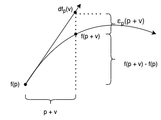
The difference function simply indicates the change in the output of \(f\) based on the input to \(f\) relative to a fixed point \(p\), i.e. how \(f\) changes as its input deviates from the point \(p\) in the direction \(v\). See Figure 1 for a one-dimensional illustration.

The difference function is non-linear in general. The differential \(df_p\) is intended to be the best linear approximation to \(\Delta_p f\).
The difference function simply measures how \(f\) varies as it deviates from point \(p\) by vector \(v\). We can then define the derivative as the best linear approximation of the difference function. That is, we want \(df_p : \mathbb{R}^n \rightarrow \mathbb{R}\) to be a linear map such that
\[\Delta_pf(v) \approx df_p(v),\]
which means that there is an exact equation
\[\Delta_pf(v) = df_p(v) + \varepsilon(v),\]
where \(\varepsilon(v)\) indicates the error, i.e. the difference between \(\Delta_pf(v)\) and its approximation \(df_p(v)\), and is thus defined as
\[\varepsilon(v) = \Delta_pf(v) - df_p(v).\]
We require that \(\varepsilon(v) \in o\left(\lVert v \rVert\right)\), that is
\[\lim_{v \to 0}\frac{\varepsilon(v)}{\lVert v \rVert} = 0.\]
This means that
\[\lim_{v \to 0}\frac{\lVert \Delta_pf(v) - df_p(v) \rVert}{\lVert v \rVert} = 0.\]
Thus, as \(v\) approaches \(0\), the difference between \(\Delta_pf(v)\) and \(df_p(v)\) vanishes "faster" than \(v\) approaches \(0\).
Expanding this definition, we recover a condition equivalent to the usual definition of the derivative:
\[\lim_{v \to 0}\frac{\lVert f(p+v) - f(p) - df_p(v) \rVert}{\lVert v \rVert} = 0.\]
The Differential in Coordinates
Now, let's examine the expression for differentials in a given coordinate system.
More generally, the differential \(df_p : T_pM \rightarrow \mathbb{R}\) can be defined on an arbitrary smooth manifold \(M\): given a tangent vector \(v : T_pM\), the differential is defined as
\[df_p(v) = v(f).\]
Recall that, given any finite-dimensional, real vector space \(V\), it dual space is the vector space \(V^*\) defined as the set of all linear functionals on \(V\), that is, the space of all linear maps \(\omega : V \rightarrow \mathbb{R}\). These linear functionals are often called covectors.
Given a basis \(E_i\) for \(V\), we can derive a corresponding dual basis \(\varepsilon^i\) for \(V^*\). Consider the action of a covector \(\omega\) on a vector \(v \in V\) represented as \(v^iE_i\) in this basis:
\[\omega\left(v^iE_i\right) = v^i\omega(E_i).\]
If we define covectors \(\varepsilon^i\) such that \(\varepsilon^i(v) = v^i\), then we obtain
\[\omega\left(v^iE_i\right) = v^i\omega(E_i) = \omega(E_i) \varepsilon^i(v).\]
This is equivalent to the requirement that \(\varepsilon(E_i) = 1\), since
\[\varepsilon(v^iE_i) = v^i\varepsilon(E_i) = v^i.\]
We often define \(\omega_i = \omega(E_i)\) and write
\[\omega = \omega_i \varepsilon^i.\]
Given smooth coordinates \((x^i)\) on a manifold, the corresponding coordinate basis \((\partial/\partial x^i \rvert_p)\) for the tangent space \(T_pM\) at a point \(p \in M\) induces a dual basis on the cotangent space \(T^*_pM\) which we will temporarily denote as \(\lambda^i \rvert_p\). Consider the action of the differential \(df_p : T_pM \rightarrow \mathbb{R}\) of a smooth function \(f : M \rightarrow p\) on a tangent vector \(v \in T_pM\) represented as \(v = v_i \partial/\partial x^i \rvert_p\) in this basis:
\begin{align}df_p(v) &= df_p\left(v^i \frac{\partial}{\partial x^i}\bigg\rvert_p\right) \\&= v^i df_p\left(\frac{\partial}{\partial x^i}\bigg\rvert_p\right) \\&= v^i \frac{\partial}{\partial x^i}\bigg\rvert_p(f) \\&= \frac{\partial f}{\partial x^i}(p) \lambda^i\rvert_p(v).\end{align}
Next, consider the special case of the differentials \((dx^i)\) of the coordinate functions themselves:
\begin{align}dx^i_p(v) &= dx^i_p\left(v^j\frac{\partial}{\partial x^j}\bigg\rvert_p\right) \\&= v^j dx^i_p\left(\frac{\partial}{\partial x^j}\bigg\rvert_p\right) \\&= v^j\frac{\partial}{\partial x^j}\bigg\rvert_p(x^i) \\&= \frac{\partial x^i}{\partial x^j}(p) \lambda^j\rvert_p(v) \\&= \delta^i_j \lambda^j\rvert_p(v) \\&= \lambda^i\rvert_p(v).\end{align}
Thus, the coordinate differentials \((dx^i\rvert_p)\) are precisely the dual basis \(\lambda^i\rvert_p\). Thus, we may instead write
\[df_p = \frac{\partial f}{\partial x^i}(p) dx^i\rvert_p.\]
If we write this in "point-free" form as a covector field, then we obtain
\[df = \frac{\partial f}{\partial x^i} dx^i.\]
This is the classical expression for the (global) differential \(df\) in coordinates. In particular, for a one-dimensional manifold, writing the basis vector field as \(d/dx\), we obtain
\[df = \frac{df}{dx}dx.\]