Metropolis Light Transport

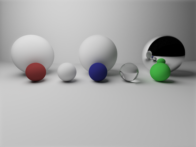
In this post, we will explore Metropolis Light Transport and the relevant theoretical background from computer graphics.

Introduction

The ultimate goal of any rendering algorithm is to produce a two-dimensional image which is a projection of a virtual, three-dimensional scene.

Ray tracing refers broadly to a class of rendering algorithms which "trace" the trajectories of "rays" of light throughout an environment. Some ray tracing algorithms are physically based, which means that they are based on certain physical principles of light. Physically based algorithms can achieve photorealism, that is, they can produce images indistinguishable from photographs. Such techniques are used for animated movies, computer-generated imagery (CGI) in feature films, television advertisements, product images in catalogs, etc.

In this post, I will describe the theory behind a rendering technique known as "Metropolis Light Transport" in addition to background information about physically based rendering.

I have implemented the algorithm described in the paper Multiplexed Metropolis Light Transport [1]. The source code, written in the Rust programming language, is available here.

The Multiplexed Metropolis Light Transport algorithm is based on the Primary Sample Space Metropolis Light Transport [2] algorithm, which is a variant of the original Metropolis Light Transport [3] algorithm, which is further detailed in this PhD thesis.

Coordinates

The virtual scene is modeled as a collection of surfaces embedded in \(\mathbb{R}^3\). The elements of \(\mathbb{R}^3\) (i.e. tuples of the form \((x,y,z)\) for some \(x,y,z \in \mathbb{R}\)) can be thought of as either points or vectors emanating from the origin (the point \((0,0,0)\)).

Given any basis \((E_1,E_2,E_3)\) for \(\mathbb{R}^3\), the coordinates of a vector \(v \in \mathbb{R}^3\) refer to the vector \((v^1, v^2, v^3)\) such that \(v = v^1E_1 + v^2E_2 + v^3E_3\). In the standard basis (\(e_1 = (1,0,0)\), \(e_2 = (0,1,0)\), and \(e_3 = (0,0,1)\)), coordinate vectors and vectors coincide (\(v = (v^1, v^2, v^3) = v^1e_1 + v^2e_2 + v^3e_3\)). The standard basis is conventionally labeled as \((e_x, e_y, e_z)\).

Orientation and Handedness

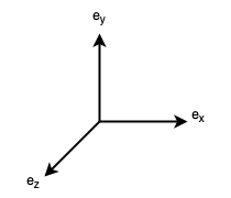
We must designate a spatial orientation for the basis vectors in order to apply them to computer graphics. For instance, the following orientation is the conventional way to spatially orient the standard basis:

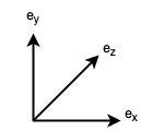
Another common spatial orientation of the basis vectors is as follows:

It is important to emphasize that this labelling of the basis vectors and spatial orientation is completely arbitrary. The notion of a spatial orientation is not a mathematical notion, but is rather a pragmatic aspect of the application of mathematics to represent objects spatially.

The orientation in Figure 2 is called a right-handed orientation, since it obeys the right-hand rule: if you point the index finger of your right hand in the direction of a vector \(a\), and the middle finger of your right hand in the direction of a vector \(b\), the cross-product \(a \times b\) (which is perpendicular to \(a\) and \(b\)) then points in the direction of the thumb of your right hand. In particular, \(e_x \times e_y = e_z\), and thus, in a right-handed orientation, if \(e_x\) points "to the right" of the screen and \(e_y\) points "to the top" of the screen, then \(e_z\) points "out of" the screen. In a right-handed orientation, positive rotation is counterclockwise about the axis of rotation.

The orientation in Figure 3 is called a left-handed orientation, since it obeys the left-hand rule: if you point the index finger of your left hand in the direction of a vector \(a\), and the middle finger of your left hand in the direction of a vector \(b\), the cross-product \(a \times b\) (which is perpendicular to \(a\) and \(b\)) then points in the direction of the thumb of your left hand. In particular, \(e_x \times e_y = e_z\), and thus, in a left-handed orientation, if \(e_x\) points "to the right" of the screen and \(e_y\) points "to the top" of the screen, then \(e_z\) points "into" the screen. In a left-handed orientation, positive rotation is clockwise about the axis of rotation.

Thus, the standard basis can be given either a right-handed or a left-handed spatial orientation.

There is a well-defined mathematical notion of the orientation of a vector space. Given a basis \(B = (E_1,E_2,E_3)\) and a basis \(B' = (E_1',E_2',E_3')\) for \(\mathbb{R}^3\), there exists a unique linear transformation \(A : \mathbb{R}^3 \rightarrow \mathbb{R}^3\) that maps \(B\) to \(B'\). If \(A\) has positive determinant, then the bases are said to be consistently oriented. If \(A\) has negative determinant, then the bases are said to be oppositely oriented. The determinant is an alternating, multilinear operation on vector spaces, and thus its sign changes with each permutation or sign change of the basis vectors, so "inverting" or "relabelling" the basis vectors will cause the sign to change. Thus, every basis can be sorted into one of two equivalence classes. By convention, the standard basis is designated as a "positive" orientation, and thus its equivalence class consists of all "positively oriented" bases, whereas the other equivalence class consists of all "negatively oriented" bases.

The notion of a spatial orientation is unrelated to the notion of the orientation of a vector space. Since the standard basis can be assigned either a right-handed or left-handed spatial orientation, yet corresponds to a unique vector space orientation, the two notions are independent. The former is a conventional and pragmatic decision made for applications of mathematics, and the latter is a precise mathematical concept. However, if we stipulate a particular spatial orientation, then we can relate the concepts. For instance, if we stipulate a right-handed spatial orientation, as in Figure 4, then, since \(e_z\) points "out of" the screen, then \(-e_z\) points "into" the screen.

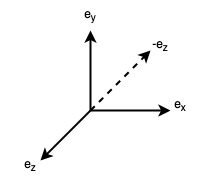
Thus, if we represent vectors using the basis \(E_x = e_x\), \(E_y = e_y\), and \(E_z = -e_z\), then, if the coordinates of a vector \(v \in \mathbb{R}^3\) are \((v^x, v^y, v^z)\) according to the standard basis, then the coordinates of \(v\) in this new basis are \((v^x, v^y, -v^z)\) since \(v = v^xE_x + v^yE_y - v^zE_z = v^xe_x + v^ye_y + v^ze_z\). In other words, we simply negate the "z" coordinate in the standard basis to determine the "z" coordinate in this new basis. Thus, in this new basis, we can use the coordinates \((0,0,2)\), for instance, to represent a vector of length \(2\) pointing "into" the screen along the "z" axis. This new basis is negatively oriented, whereas the standard basis is positively oriented (by convention). Thus, the two spatial orientations correspond to two vector space orientations, but only if we first arbitrarily stipulate a particular spatial orientation in the context of some application.

For instance, sometimes it is asserted that a right-handed orientation is one in which \(E_x \times E_y = E_z\) and a left-handed orientation is one in which \(E_x \times E_y = -E_z\). However, the standard basis (in which \(e_x \times e_y = e_z\)) can be assigned both a right-handed and a left-handed spatial orientation. The mathematical equivalence \(e_x \times e_y = e_z\) is true regardless of how we spatially depict vectors. This assertion is based on the assumption that a right-handed spatial orientation has been stipulated (and therefore cannot define right-handedness, since such a definition would be circular). In the example of the basis above (where \(E_z = -e_z\)), it is indeed the case that \(E_x \times E_y = -E_z\) (since \(E_x \times E_y = e_x \times e_y = e_z = -E_z\)). However, we only chose such a basis based on our arbitrary conventions about the labelling and spatial orientation of the basis vectors. Mathematically, the cross product is independent of spatial orientation. However, once we have designated a spatial orientation, the corresponding rule (right-hand or left-hand rule) will enable us to remember which way the cross product must point when interpreted according to our conventions.

Thus, we simply need to designate our desired convention for spatial orientation, and we can use the appropriate rule (right-hand or left-hand) as a practical device for determining the spatial orientation corresponding to the results of various mathematical operations (such as the cross product or rotations).

In this post, I use the left-handed convention, that is, we label the "x" direction as pointing to the "right" of the screen, the "y" axis as pointing to the "top" of the screen, and the "z" axis as pointing "into" the screen. I initially chose this orientation because the renderer PBRT uses this same convention, and I used it as a reference.

Local Coordinates

It is very useful to use local coordinates in many situations. For instance, when considering a ray intersection at a point on a surface, it is convenient to represent the normal vector at this point as the vector \((0,0,1)\). A transformation (typically in matrix form) will transform the global coordinates of any inputs the local coordinates, and an inverse transformation will transform the local coordinates of any computed results back to global coordinates.

As an example, consider Figure 5.

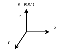
If the normal vector is always expressed as \(n = (0,0,1)\), then many calculations are substantially simplified. For instance, to determine if a given vector is in the same hemisphere as the normal vector, it is sufficient to check that the \(z\) component of the vector is positive. The dot product of a vector with the normal is equal to the \(z\) component of the vector. The reflection a vector \((v^x,v^y,v^z)\) across the normal is simply the vector \((-v^x,-v^y,v^z)\).

The prototype implementation linked above does not use local coordinates, but local coordinates are generally preferable.

Geometry

Objects in the scene are generally modeled as implicit surfaces. For instance, spheres are modeled as solutions to the equation

\[\lVert p - o \rVert = R,\]

where \(p\) represents any point on the surface of the sphere, \(o\) represents the location of the center of the sphere, and \(R\) represents the radius of the sphere. Thus, a sphere is completely determined by specifying its center and radius.

The (unit) normal vector at any point \(p\) on the surface of a sphere can be computed as

\[n_p = \frac{p - o}{\lVert p - o \rVert} = \frac{p-o}{R}.\]

The normal vector is one which is orthogonal to all of the tangent vectors at the point.

A ray is the combination of a point \(r_o\) (the "origin" of the ray) and a unit vector \(r_d\) (the "direction" of the ray). Thus, a ray is like a vector, but translated to a different origin.

Our primary task is to determine the closest object (if any) that a ray intersects.

Spheres

Let us consider how to determine if a ray intersects a sphere. Consider Figure 6.

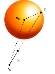
We denote the sphere's center (origin) as \(s_o\) and radius as \(R\). We want to determine the the point \(p\) on the surface of the sphere (if any) that the ray intersects. We want to determine how far we need to extend the ray in order to intersect the sphere. Thus, we want to determine the scalar \(t \in \mathbb{R}\) such that

\[p = r_o + t r_d.\]

We employ the Law of Cosines, which indicates that, for a leg with length \(a\) and opposite angle \(\alpha\) and additional legs with lengths \(b\) and \(c\) which comprise a triangle,

\[a^2 = b^2 + c^2 - 2ab \cos \alpha.\]

Thus, we have a triangle with legs of the following lengths:

• \(R = \lVert p - s_o \rVert\),
• \(t = \lVert p - r_o \rVert = \lVert (r_o + t r_d) - r_o \rVert = \lVert t r_d \rVert = t \lVert r_d \rVert = t\) (since \(r_d\) is a unit vector),
• \(\lVert s_o - r_o \rVert\).

The angle \(\alpha\) opposite the leg with length \(R\) is then calculated as

\[\cos \alpha = \frac{s_o - r_o}{\lVert s_o - r_o \rVert} \cdot r_d\]

since the cosine of the angle between two unit vectors is computed by their dot product. Thus, the Law of Cosines yields the following equation:

\begin{align}R^2 &= t^2 + \lVert s_o - r_o \rVert^2 - 2 t \lVert s_o - r_o \rVert \frac{s_o - r_o}{\lVert s_o - r_o \rVert} \cdot r_d \\&= t^2 + \lVert s_o - r_o \rVert^2 - 2 t (s_o - r_o) \cdot r_d .\end{align}

Thus, we also infer that

\[t^2 - (2 (s_o - r_o) \cdot r_d) t + (\lVert s_o - r_o \rVert^2 - R^2) = 0.\]

Applying the Quadratic Formula, we obtain the following:

\begin{align}t &= \frac{-(-2(s_o - r_o) \cdot r_d) \pm \sqrt{(-2(s_o - r_o) \cdot r_d)^2 - 4(\lVert s_o - r_o \rVert^2 -R^2)}}{2} \\&= \frac{(2(s_o - r_o) \cdot r_d) \pm \sqrt{4((s_o - r_o) \cdot r_d)^2 + 4(R^2 - \lVert s_o - r_o \rVert^2)}}{2} \\&= \frac{(2(s_o - r_o) \cdot r_d) \pm \sqrt{4(((s_o - r_o) \cdot r_d)^2 + R^2 - \lVert s_o - r_o \rVert^2)}}{2} \\&= \frac{(2(s_o - r_o) \cdot r_d) \pm 2\sqrt{((s_o - r_o) \cdot r_d)^2 + R^2 - \lVert s_o - r_o \rVert^2}}{2} \\&= ((s_o - r_o) \cdot r_d) \pm \sqrt{((s_o - r_o) \cdot r_d)^2 + R^2 - \lVert s_o - r_o \rVert^2}.\end{align}

Thus, if the radicand is negative, there is no solution, and the ray does not intersect the sphere. The scalar \(t\) should be positive since the ray is supposed to project "forward" and not "backward". Thus, the positive solution (if any) is used. Otherwise, the ray does not intersect the sphere.

Acceleration Structures

The object that a ray intersects is the closest object intersected by a ray. For simple scenes with only a few objects, it is sufficient to test every object for intersection, then select the closest object (i.e. minimum value of \(t\)). For more complex scenes, an acceleration structure will be required for intersection tests to be computationally tractable, such as a bounding volume hierarchy which permits a subset of the objects to be tested efficiently.

Camera Models

We require a camera model which simulates a camera which captures an image of the scene.

Pinhole Camera Model

The simplest camera model is the pinhole camera. A pinhole camera consists of an opaque enclosure with a tiny aperture (the "pinhole") on one end and a film or sensor on the opposite end, as depicted in Figure 7. A pinhole camera produces an inverted image since light entering the pinhole from above will ultimately strike the film below, etc.

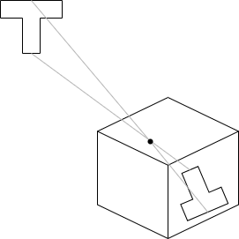
The virtual pinhole camera is depicted in Figure 8.

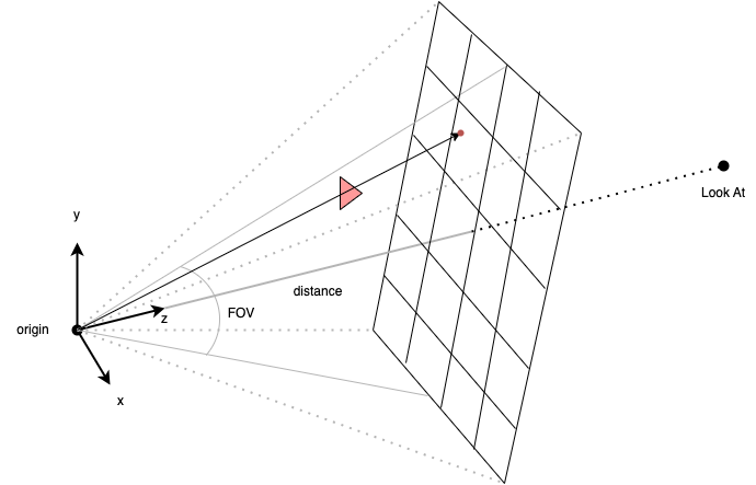
A pinhole camera model is specified by the following data:

• The origin - a point which corresponds to the "pinhole".
• The target (or look at) point - a point which determines the direction in which the camera will point.
• The vertical field of view - the measure of the angle formed by two vectors emanating from the origin, enclosed within the y-z plane, and terminating at the top and bottom of the image, respectively.
• The width and height of the image, in pixels, which also corresponds to the width and height of the image within the coordinate system used to represent the virtual scene.

From this data, the following data is then computed:

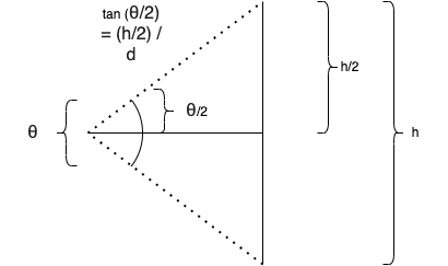
• The distance from the origin to the image, computed as \[\frac{h}{2 \tan \left(\frac{\theta}{2}\right)},\] where \(h\) represents the image height and \(\theta\) represents the field of view (see Figure 9). The distance represents the length of the adjacent leg of a right triangle, relative to the angle \(\theta/2\), whose opposite leg has length \(h/2\), and thus \(\tan (\theta/2) = (h/2)/d\), where \(d\) represents the distance.
• An orthonormal basis for a vector space centered at the origin. This basis determines a coordinate system relative to the camera. First, the "z" basis vector \(c_z\) is computed as \(\frac{t - o}{\lVert t - o \rVert}\), where \(o\) represents the origin and \(t\) represents the target (or "look at") point. The "z" axis thus points from the origin to the target. It is normalized by dividing by its length. Since the cross product of two linearly independent vectors in \(\mathbb{R}^3\) represents a vector which is orthogonal to each of the two vectors, and since we have adopted a left-handed convention, the "x" basis vector can be computed as \(c_x = e _y \times c_z\) if \(c_z\) and \(e_y\) are linearly independent. Then, the "y" basis vector can be computed as \(c_x = c_z \times c_x\). Otherwise, if \(c_z\) and \(e_y\) and linearly dependent, then the "y" basis vector can be computed as \(c _y = e_x \times c_z\) and then the "x" basis vector can be computed as \(c_x = c_y \times c_z\).

Note that the rectangular region representing the image is in front of the origin in the virtual camera model (whereas the film is behind the pinhole in a real pinhole camera) which thus produces an image which is not inverted. The origin forms the apex of a pyramid whose edges pass through the corners of the image region and extends indefinitely; this pyramid is called the view frustum. Any portion of an object situated within the view frustum is potentially visible in the image (but may be occluded by some other object), and any portion of any object situated outside the view frustum is not visible in the image. For instance, Figure 7 depicts a red triangle that lies entirely within the view frustum, and a red dot which indicates which pixel corresponds to a particular ray which intersects the triangle. It does not matter whether an object is in front of or behind the image region since the image region has no physical significance, but rather is positioned solely for the purpose of calculating the pixel coordinates of the intersection points of rays with the image region. Each pixel represents a \(1 \times 1\) square region within the image rectangle relative to the coordinate system.

Solid Angle

Before discussing solid angle, it is useful to review the concept of planar angle.

A planar angle is a geometric figure consisting of a point, called a vertex, and two line segments which share the vertex as a common endpoint, as in Figure 10. The angle subtended by a segment of a curve is the angle formed between a given vertex and two line segments extending from the vertex to two given points on the curve, as in Figure 9. As Figure 9 also indicates, an important special case is when the curve that subtends an angle is an arc (i.e. a segment of a circle).

Various measures can be defined to express the magnitude of an angle. For instance, the unit of radians expresses the ratio of arc length to radius relative to a particular circle. One radian is the measure of the angle subtended by an arc on a particular circle whose length is equal to the radius of the same circle. Thus, on the unit circle (i.e. the circle with radius \(1\)), the angular measurement in radians expresses the length of the arc that subtends the angle. Thus, in units of radians, the angular measure of the projection (i.e. arc) of a curve onto a circle of a given radius is equivalent to the angular measure of the projection of the curve onto the unit circle.

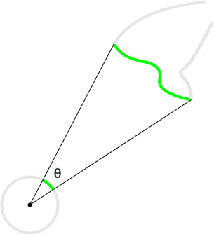
Solid angle is the generalization of planar angle to three dimensions. When restricted to spheres, solid angle can be conceived as a geometric figure which resembles a cone terminating in a spherical cap, as in Figure 11.

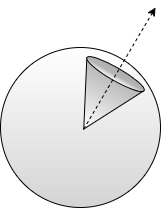
However, due to the difficulty of defining such a figure precisely for more general surfaces, we only define the measure of solid angle (and often simply refer to this measure as "solid angle"). Just as the measure of the planar angle subtended by a curve is the measure of the arc length of the projection of a curve onto the unit circle, the measure of solid angle is analogously the measure of the area of the projection of an arbitrary surface onto the unit sphere, as in Figure 12. The surface is said to subtend the solid angle at the given apex (center of the unit sphere). Unlike planar angle, where the projection of a curve onto the unit circle is always in the shape of an arc, the projection of a surface onto the unit sphere can assume an arbitrary shape. This is analogous to the "shadow" of the shape.

The measure of solid angle is expressed in units of steradians. One steradian is defined as the ratio of the area of the solid angle subtended by a given surface at the center of a given sphere to the square of the radius of the sphere (since the surface area of a sphere is proportional to the square of its radius). Thus, on a unit sphere (i.e. the sphere with radius \(1\)), the unit of steradians measures the area of the solid angle subtended by a surface. In other words, on the unit sphere, the unit of steradians measures the area of the projection of the surface onto the unit sphere.

Throughout our discussion, we will make several simplifying assumptions so that these details will not serve as a distraction:

1. We are only considering a single surface.
2. The entirety of the surface is "visible" from the given apex (i.e. there are no "folds" of the surface which are occluded by another portion of the surface).
3. No other intermediate object occludes the surface (there is no object between the apex and each point on the surface under consideration).
4. We will neglect the fact that the scene might be open (i.e. the surface of the unit sphere might not be completely covered by projections from other surfaces).

We will relax these assumptions after we introduce numerical integration.

Thus, we need to be able to calculate this projection for arbitrary surfaces. Figure 13 depicts the approximation to the projection at a point.

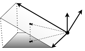
Each surface \(S\) has a parameterization \(r(s,t) : T \rightarrow S\), where \(T\) is a Euclidean (flat, rectangular) domain (rectangular subset of \(\mathbb{R}^2\)). At each point \(p\) on the surface, we define a facet which approximates the area of the surface near the point. This facet is a parallelogram spanned by the tangent vectors \(\partial/\partial s\rvert_p\) and \(\partial/\partial t\rvert_p\) emanating from the point \(p\). We can also define the normal vector at the point as \(\mathbf{n}_p = \partial/\partial s\rvert_p \times \partial/\partial t\rvert_p\). Every point on the facet is orthogonal to \(\mathbf{n}_p\) and \(\mathbf{n}_p\) is orthogonal to both \(\partial/\partial s\rvert_p\) and \(\partial/\partial t\rvert_p\). We fix a given apex \(o\) and consider the sphere with center \(o\) and radius \(\lVert p - o \rVert\) so that the point \(p\) also lies on the surface of this sphere. We want to define the area of the projection of this facet onto a plane that is tangent at this point to this sphere. We can also define a unit vector \(N(p)\) normal to the sphere at this point (and hence normal to the tangent plane at this point also). The angle between \(N(p)\) and \(\mathbf{n}_p\) is the same as the angle between each point on the facet and its projection onto the tangent plane. Since the magnitude of the cross product of any two vectors is equal to the area of the parallelogram spanned by the vectors, the cross product \(\mathbf{n}_p = \partial/\partial s\rvert_p \times \partial/\partial t\rvert_p\) of the facet's spanning vectors has a magnitude which is equal to the area of the facet. Thus, in a sense, \(\mathbf{n}_p\) represents the facet and \(N(p)\) represents the tangent plane. Thus, the magnitude of the projection of \(\mathbf{n}_p\) onto \(N(p)\) is equal to the area of the projection of the facet onto a plane tangent to the sphere. This projection can be computed via the dot product as

\[\left(\frac{\partial}{\partial s}\bigg\rvert_p \times \frac{\partial}{\partial t}\bigg\rvert_p\right) \cdot N(p) = \left\lVert \frac{\partial}{\partial s}\bigg\rvert_p \times \frac{\partial}{\partial t}\bigg\rvert_p\right\rVert \lVert N(p) \rVert \cos \theta_p = \left\lVert \frac{\partial}{\partial s}\bigg\rvert_p \times \frac{\partial}{\partial t}\bigg\rvert_p \right\rVert \cos \theta_p,\]

where \(\theta_p\) is the measure of the angle between the normal vectors, and is thus defined such that

\[\cos \theta_p = N(p) \cdot \frac{\frac{\partial}{\partial s}\bigg\rvert_p \times \frac{\partial}{\partial t}\bigg\rvert_p}{\bigg\lVert\frac{\partial}{\partial s}\bigg\rvert_p \times \frac{\partial}{\partial t}\bigg\rvert_p\bigg\rVert}.\]

The unit vector normal to a sphere with center \(o\) at point \(p\) is defined as

\[N(p) = \frac{p - o}{\lVert p - o \rVert}.\]

The radius of the sphere at point \(p\) is thus defined as

\[R_p = \lVert p - o \rVert.\]

Since the measure of solid angle on the sphere is the ratio of this projection to the square of the radius of the sphere, the measure of the solid angle is thus

\[\frac{1}{R_p^2}\left(\frac{\partial}{\partial s}\bigg\rvert_p \times \frac{\partial}{\partial t}\bigg\rvert_p\right) \cdot N(p) = \frac{1}{R_p^2}\left\lVert \frac{\partial}{\partial s}\bigg\rvert_p \times \frac{\partial}{\partial t}\bigg\rvert_p \right\rVert\cos \theta_p.\]

Thus, if we define a vector field \(F : S \rightarrow \mathbb{R}^2\) as

\[F(p) = \frac{1}{R_p^2}N(p),\]

then the surface integral of this vector field computes the solid angle as

\begin{align}\iint_S F \cdot ~d\mathbf{s} &= \iint_S F \cdot \mathbf{n} ~ds \\&= \iint_T F(r(s,t)) \cdot \left(\frac{\partial}{\partial s}\bigg\rvert_{r(s,t)} \times \frac{\partial}{\partial t}\bigg\rvert_{r(s,t)}\right) ~ds~dt.\end{align}

We can also write this integral as

\begin{align}\iint_T F(r(s,t)) \cdot \left(\frac{\partial r}{\partial s} \times \frac{\partial r}{\partial t} \right) ~ds~dt &= \iint_T \frac{1}{R_{(s,t)}^2}N(r(s,t))\cdot \left(\frac{\partial r}{\partial s}\bigg\rvert_{r(s,t)} \times \frac{\partial r}{\partial t}\bigg\rvert_{r(s,t)} \right) ~ds~dt \\&= \iint_T \frac{1}{R_{r(s,t)}^2}N(r(s,t))\cdot \frac{\left(\frac{\partial r}{\partial s}\bigg\rvert_{r(s,t)} \times \frac{\partial r}{\partial t}\bigg\rvert_{r(s,t)} \right)}{\bigg\lVert \frac{\partial r}{\partial s}\bigg\rvert_{r(s,t)} \times \frac{\partial r}{\partial t}\bigg\rvert_{r(s,t)} \bigg\rVert } \bigg\lVert \frac{\partial r}{\partial s} \times \frac{\partial r}{\partial t}\bigg\rvert_{r(s,t)}\bigg\rVert ~ds~dt \\&= \iint_T \frac{1}{R_{r(s,t)}^2}\cos \theta_{r(s,t)} \left\lVert \frac{\partial r}{\partial s}\bigg\rvert_{r(s,t)} \times \frac{\partial r}{\partial t}\bigg\rvert_{r(s,t)} \right\rVert ~ds~dt. \end{align}

Thus, if we define a scalar field \(F : T \rightarrow \mathbb{R}\) as

\[F(p) = \frac{1}{R_p^2} \cos \theta_p\],

then this integral also computes the integral of this scalar field:

\begin{align}\iint_S F dS &= \iint_T F(r(s,t)) \bigg\rVert \frac{\partial r}{\partial s}\bigg\rvert_{r(s,t)} \times \frac{\partial r}{\partial t}\bigg\rvert_{r(s,t)} \bigg\lVert~ds~dt \\&= \iint_T \frac{1}{R_{r(s,t)}^2}\cos \theta_{r(s,t)} \left\lVert \frac{\partial r}{\partial s}\bigg\rvert_{r(s,t)} \times \frac{\partial r}{\partial t}\bigg\rvert_{r(s,t)} \right\rVert ~ds~dt .\end{align}

The integral over this scalar field is often abbreviated as

\[\int_A \frac{1}{R^2}\cos \theta ~dA.\]

In this abbreviation, the \(A\) represents "area", and the parameters are suppressed, i.e. \(\theta\), \(R\), and \(\omega\) are functions that compute values for each point on the surface. This notation is employed since it is economical.

This defines a particular volume measure which can be used for integrating functions.

Thus, given any function \(f : S \rightarrow \mathbb{R}\), we define the integral with respect to surface area as

\begin{align}\iint_S f~dS &= \iint_S f (\frac{1}{R^2} \cos \theta) dS \\&= \iint_T f(r(s,t)) \frac{1}{R_{r(s,t)}^2} \cos \theta_{r(s,t)} \left\lVert \frac{\partial r}{\partial s}\bigg\rvert_{r(s,t)} \times \frac{\partial r}{\partial t}\bigg\rvert_{r(s,t)} \right\rVert ~ds ~dt.\end{align}

The integral with respect to solid angle is simply the integral of a function whose support is precisely the solid angle of some surface (i.e. the projection of the surface onto the unit sphere) over the unit sphere (see this post for a derivation):

\begin{align}\iint_\Omega f ~d\omega = \int_0^{2\pi}\int_0^{\pi} f(r(\varphi,\theta)) \sin \varphi ~d\varphi~d\theta.\end{align}

In other words, \(f(p) = 0\) for any point \(p\) outside the projection of the surface onto the unit sphere, and \(f(p)\) is only non-zero within the projection.

We can compute the point \(\omega(p)\) on the unit sphere with center \(o\) corresponding to a point \(p\) on a surface \(S\) as

\[\omega(p) = \frac{p - o}{\lVert p - o \rVert}.\]

Given a function \(f\) defined on the unit sphere, we can convert to an integral over area as follows:

\begin{align}\iint_\Omega f ~d\omega &= \iint_S f(\omega) (\frac{1}{R^2} \cos \theta) dS \\&= \iint_T f(\omega(r(s,t)) \frac{1}{R_{r(s,t)}^2} \cos \theta_{r(s,t)} \left\lVert \frac{\partial r}{\partial s}\bigg\rvert_{r(s,t)} \times \frac{\partial r}{\partial t}\bigg\rvert_{r(s,t)} \right\rVert ~ds ~dt.\end{align}

This equivalence is often abbreviated as

\[\int_{\S^2} f ~d\omega = \int_{A}f(\omega) \frac{1}{R^2}\cos \theta~dA.\]

Thus, both integrals are related to solid angle, but one performs the integration over the unit sphere as a domain, and the other performs the integration over the surface as a domain. There is a geometric conversion factor of \(\cos \theta / R^2\) which accounts for the projection; this is not a Jacobian determinant (found in change of variables formulas from calculus).

Let's consider a simple example. Let's compute the solid angle of a sphere with radius \(2\) (as projected on a unit sphere centered at the same apex). It should cover the entire unit sphere, and hence be equal to the surface area of the unit sphere, which is \(4\pi\). If we denote the unit sphere as \(S^2\) and the sphere with radius \(2\) as \(A\) and the parameterization of \(S^2\) in terms of spherical coordinates as \(r(s,t)\), then, since \(R\) is \(2\) at each point and \(\cos \theta\) is \(1\) at each point (since the respective unit normal vectors coincide and the angle between them is \(0\) radians), we compute

\begin{align}\int_{S^2} d\omega &= \int_{A} \frac{1}{R^2}\cos \theta dA \\&= \int_0^{2\pi}\int_0^{\pi} \frac{1}{R_{r(s,t)}^2} \cos \theta_{r(s,t)} R^2 \sin s ~ds ~dt \\&= \int_0^{2\pi}\int_0^{\pi} \sin s ~ds ~dt \\&= 4\pi.\end{align}

Of course, we could have computed the surface area of the sphere with radius \(2\) directly; this calculation is simply a verification that shows that we have computed the projection correctly in this instance.

Numerical Integration

Unfortunately, it is intractably difficult (if not impossible) to determine a parameterization, since the surfaces can be arbitrarily complex and the parameterization must vary from point to point in the scene (since it must consider the "visibility" of each surface from a given apex).

However, it is quite straightforward to sample points which are visible from a given apex: simply cast a ray from the point in the appropriate direction and calculate the nearest surface (if any) that the ray intersects.

This means that we must compute the integrals numerically (that is, using a computer) rather than analytically.

There are many techniques for numerical integration. However, the only technique suitable for the high-dimensional integrals used in rendering is Monte Carlo integration.

Suppose we wish to estimate the integral

\[\int_D f(\bar{x})~d\bar{x},\]

where \(D \subseteq \mathbb{R}^n\) is some domain of integration. Suppose further that we have a set \(X\) of (real-valued) random variables, each of which has a corresponding probability density function (PDF) \(p\).

Recall that the expected value of a random variable is the continuous analog of a mean:

\[E[f] = \int_D f(\bar{x})p(\bar{x})~d\bar{x}.\]

The Monte Carlo estimator \(E_p[f]\), where \(X\) is a set of random variables drawn from a probability density function (PDF) \(p\) and \(f\) is a function, is defined as

\[E_p[f] = \frac{1}{\lvert X \rvert}\sum_{\bar{x} \in X}\frac{f(\bar{x})}{p(\bar{x})}.\]

The expected value of the estimator is exactly equal to the integral:

\begin{align}E\left[E_p[f]\right] &= E\left[\frac{1}{\lvert X \rvert}\sum_{\bar{x} \in X}\frac{f(\bar{x})}{p(\bar{x})}\right] \\&= \int_D \frac{1}{\lvert X \rvert}\sum_{\bar{x} \in X}\frac{f(\bar{x})}{p(\bar{x})} p(\bar{x}) ~d\bar{x}\\&= \frac{1}{\lvert X \rvert} \lvert X \rvert \int_Df(\bar{x}) ~d\bar{x} \\&= \int_D f(\bar{x}) ~d\bar{x}.\end{align}

We can interpret this as meaning that the estimator "on average" computes the correct value. Not only this, but the variance reduces as the sample size is increased.

The variance of a random variable \(Y\) is defined as

\[\sigma^2(Y) = E[(Y - E[Y])^2].\]

In other words, it measures the "average" squared error.

We can infer certain properties of expected values and variances; for any constant \(a\),

\[E[aY] = aE[Y],\]

\[\sigma^2(aY) = a^2\sigma^2(Y).\]

Also,

\[E[\sum_{i=1}^nY_i] = \sum_{i=1}^nE[Y_i],\]

and if the random variables are uncorrelated (independent), we can likewise infer that

\[\sigma^2[\sum_{i=1}^nY_i] = \sum_{i=1}^n\sigma^2[Y_i].\]

Then, using the random variables \(Y_i = f(X_i)/p(X_i)\), we see that the variance of the Monte Carlo estimator is given by

\begin{align}\sigma^2(E_p[f]) &= \sigma^2\left(\frac{1}{n}\sum_{i=1}^nY_i\right) \\&= \frac{1}{n^2}\sum_{i=1}^n\sigma^2(Y_i) \\&= \frac{1}{n^2}\sum_{i=1}^n\sigma^2(Y) \\&= \frac{1}{n^2}\cdot n \cdot \sigma^2(Y) \\&= \frac{1}{n}\sigma^2(Y),\end{align}

where \(\sigma^2(Y)\) represents their common variance, since each random variable has the same distribution. Then, error, being the square root of variance, is given by

\[\sigma(E_p[f]) = \frac{\sigma(Y)}{\sqrt{n}}.\]

Thus, in order to decrease the error by a factor of \(n\), the number of samples must increase by a factor of \(n^2\).

Variance manifests in rendered images as a visual artifact called noise, which is a grainy speckling of the image. As the number of samples increases, the noise decreases, and the image becomes progressively sharper and less speckled. Often, thousands of samples per pixel are required to produce acceptable results. However, there are various denoising algorithms which can remove noise from images, requiring fewer samples per pixel.

Next, let's consider the application of Monte Carlo integration to surface integrals.

Given any top-level differential form (integrand) in coordinates and a smooth map \(F\) between manifolds, the pullback is computed as follows:

\[F^*(u~dy_1 \wedge \dots \wedge dy_n) = (u \circ F)(\mathrm{det} DF)~dx_1 \wedge \dots \wedge dx_n,\]

where \(DF\) is the Jacobian matrix of \(F\) in the given coordinates. In particular, PDFs are subject to the normalization constraint that

\[\int_D p(\bar{x})~d\bar{x} = 1.\]

Thus, we see that

\begin{align}\int_S p~dy_1 \wedge \dots \wedge dy_n &= \int_D F^*(p~dy_1 \wedge \dots \wedge dy_n) \\&= \int_D (p \circ F)(\mathrm{det} DF)~dx_1 \wedge \dots \wedge dx_n \\&= \int_D (p \circ F)(\mathrm{det} DF)~dx_1 \dots dx_n \\&= \int_D (p \circ F)(\mathrm{det} DF)~d\bar{x} \\&= 1.\end{align}

Thus, we can derive a new PDF \(F^*p\) defined as

\[F^*p(\bar{x}) = p(F(\bar{x}))(\mathrm{det} DF).\]

For a parameterization \(r(s,t) : D \rightarrow S\) of some surface \(S\), since

\[\mathrm{det}(Dr) = \bigg\lVert \frac{\partial}{\partial s}\bigg\rvert_{r(s,t)} \times \frac{\partial}{\partial t}\bigg\rvert_{r(s,t)} \bigg\rVert,\]

it follows that

\[r^*p(s,t) = p(s,t) ~\bigg\lVert \frac{\partial}{\partial s}\bigg\rvert_{r(s,t)} \times \frac{\partial}{\partial t}\bigg\rvert_{r(s,t)} \bigg\rVert.\]

Thus, we compute

\begin{align}E_{r^*p}[(f \circ r)(\mathrm{det} Dr)] &= \frac{1}{\lvert X \rvert}\sum_{(s,t) \in X}\frac{f(r(s,t))}{r^*p(s,t)}\bigg\lVert \frac{\partial}{\partial s}\bigg\rvert_{r(s,t)} \times \frac{\partial}{\partial t}\bigg\rvert_{r(s,t)} \bigg\rVert\\&= \frac{1}{\lvert X \rvert}\sum_{(s,t) \in X}\frac{f(r(s,t))}{p(r(s,t)) \bigg\lVert \frac{\partial}{\partial s}\bigg\rvert_{r(s,t)} \times \frac{\partial}{\partial t}\bigg\rvert_{r(s,t)} \bigg\rVert}\bigg\lVert \frac{\partial}{\partial s}\bigg\rvert_{r(s,t)} \times \frac{\partial}{\partial t}\bigg\rvert_{r(s,t)} \bigg\rVert\\&= \frac{1}{\lvert X \rvert}\sum_{(s,t) \in X}\frac{f(r(s,t))}{p(r(s,t))}.\end{align}

Thus, the \(\lVert \partial/\partial s\rvert_{r(s,t)} \times \partial/\partial t\rvert_{r(s,t)} \rVert\) term cancels out and the estimator assumes a simplified form.

The expected value of the estimator is

\begin{align}E[E_{r^*p}[(f \circ r)(\mathrm{det} Dr)]] &= E\left[\frac{1}{\lvert X \rvert}\sum_{(s,t) \in X}\frac{f(r(s,t))}{p(r(s,t))}\right] \\&= \int_D \frac{1}{\lvert X \rvert}\sum_{(s,t) \in X}\frac{f(r(s,t))}{p(r(s,t))} r^*p(s, t)~ds~dt \\&= \int_D \frac{1}{\lvert X \rvert}\sum_{(s,t) \in X}\frac{f(r(s,t))}{p(r(s,t))} p(r(s,t))\bigg\lVert \frac{\partial}{\partial s}\bigg\rvert_{r(s,t)} \times \frac{\partial}{\partial t}\bigg\rvert_{r(s,t)} \bigg\rVert ~ds~dt \\&= \int_D \frac{1}{\lvert X \rvert}\sum_{(s,t) \in X}f(r(s,t))\bigg\lVert \frac{\partial}{\partial s}\bigg\rvert_{r(s,t)} \times \frac{\partial}{\partial t}\bigg\rvert_{r(s,t)} \bigg\rVert ~ds~dt \\&= \frac{1}{\lvert X \rvert}\sum_{(s,t) \in X} \int_D f(r(s,t))\bigg\lVert \frac{\partial}{\partial s}\bigg\rvert_{r(s,t)} \times \frac{\partial}{\partial t}\bigg\rvert_{r(s,t)} \bigg\rVert ~ds~dt \\&= \frac{1}{\lvert X \rvert}\lvert X \rvert \int_D f(r(s,t))\bigg\lVert \frac{\partial}{\partial s}\bigg\rvert_{r(s,t)} \times \frac{\partial}{\partial t}\bigg\rvert_{r(s,t)} \bigg\rVert ~ds~dt \\&= \int_D f(r(s,t))\bigg\lVert \frac{\partial}{\partial s}\bigg\rvert_{r(s,t)} \times \frac{\partial}{\partial t}\bigg\rvert_{r(s,t)} \bigg\rVert ~ds~dt.\end{align}

Thus, the expected value of this estimator is indeed the surface integral.

The parameterization can be suppressed (the samples can be drawn from the set \(\{r(s,t) \mid (s,t) \in X\}\)). Then, we can simply write

\[E_p[f] = \frac{1}{\lvert X \rvert}\sum_{\bar{x} \in X}\frac{f(\bar{x})}{p(\bar{x})}.\]

Now let's return to the technical problems related to solid angle. They are:

1. There may be multiple surfaces.
2. Parts of surfaces may not be "visible" from the apex.
3. Parts of surfaces might be occluded by other surfaces.
4. Part of the surface of the unit sphere might not contain any projection from any other surface.

Numerical integration solves each of these problems. In the context of ray tracing, rays cast from the apex will determine which points to sample, and therefore only points that are "visible" from the apex will be considered, which solves the problems related to visibility.

The union of all surfaces in a scene constitutes a surface itself. There is a tacit assumption in rendering that this total scene surface can be parameterized by one or more parameterizations, even though it is not possible to state them explicitly (they are implicit, however, in the ray tracing, which represents an implicit parameterization of the total scene surface).

To understand the fourth problem, consider an example as in Figure X. Suppose that we want to compute some PDF with respect to solid angle expressed over the unit sphere at a point. This PDF must integrate to \(1\) over the entire surface of the unit sphere. When converting this PDF to a PDF with respect to surface area, we are tacitly assuming that the entire surface of the unit sphere contains the projection of some surface, which might not be true. However, we can conceptualize this issue as if there were a spherical surface which encapsulates the entire scene as in Figure X. Then, ray "misses" (i.e. when a ray does not intersect any object in the scene) correspond implicitly to points along this hypothetical surface.

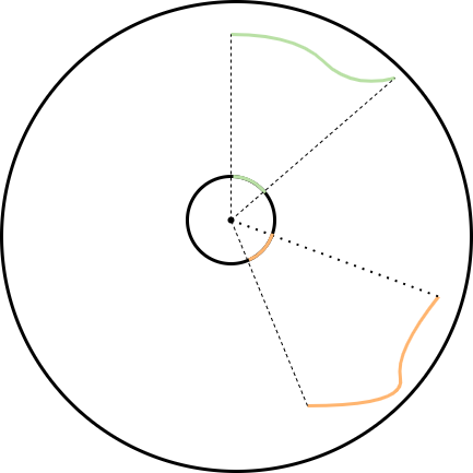
Thus, the Monte Carlo estimator with respect to area is defined as

\[\int_Af~dA \approx E_{p}[f] = \frac{1}{\lvert X \rvert}\sum_{\bar{x} \in X}\frac{f(\bar{x})}{p(\bar{x})}.\]

Likewise, the Monte Carlo estimator with respect to solid angle is defined as

\[\int_{S^2}f~d\omega \approx E_{p}[f] = \frac{1}{\lvert X \rvert}\sum_{\bar{x}\in X}\frac{f(\bar{x})}{p(\bar{x})}.\]

This is just a special case of an integral with respect to area, in which it is typically assumes that the support of the function \(f\) corresponds to the solid angle subtended by some surface.

The conversion from solid angle to area is defined such that

\[\int_{S^2}f~d\omega = \int_A f(\omega) \frac{1}{R^2}\cos \theta~dA \approx \frac{1}{\lvert X \rvert}\sum_{\bar{x} \in X}\frac{f(\omega(\bar{x}))}{p(\bar{x})}\frac{1}{R^2_{\bar{x}}}\cos \theta_{\bar{x}}.\]

Delta Distributions

In rendering, certain functions arise whose support (the set of points where the function is non-zero) is a single point. For instance, the reflectance function (BRDF) for perfect specular reflection ("mirror" reflection) is only non-zero for a single pair of directions (the reflection across the normal at a point).

This causes problems for defining integrals. One approach would be to attempt to use the Dirac measure and Lebesgue integration. However, a very effective approach in the context of rendering uses the theory of distributions.

Formally, a distribution is a continuous linear functional on \(C^k_c(U)\), the space of all \(k\)-times differentiable functions with signature \(U \rightarrow \mathbb{R}\) with compact support in \(U\) (where \(C^k_c(U)\) is endowed with a certain canonical topology called the canonical LF topology).

Informally, a distribution \(f\) "acts" on "test functions" \(\psi\) by "sending" each test function to a real number \(D_f(\psi)\), also denoted \(f[\psi]\); the value \(D_f(\psi) = f[\psi]\) is typically interpreted as the result of "integration" with respect to a test function \(\psi\), and is thus often denoted as

\[\int_{\mathbb{R}^n} f(\bar{x})\psi(\bar{x}) d\bar{x} = D_f(\psi).\]

Note that this is a definitional equality, i.e. the left-hand side is simply notation (it does not typically correspond to an integral defined in any ordinary sense) and the right-hand side is stipulated as the definition of the left-hand side. The notation looks like the "convolution" of the distribution \(f\) with the function \(\psi\) since it places them side by side.

The Dirac delta distribution \(\delta_a\) is defined such that, for any test function \(\psi : U \rightarrow \mathbb{R}\) (where \(U \subset \mathbb{R}^n\)),

\[\delta_a[\psi] = \psi(a).\]

Thus, the Dirac delta distribution acts on test functions by sending them to their value at a given point \(a\). Thus, using the notation introduced earlier,

\[\int_{\mathbb{R}^n} \delta_a(\bar{x})\psi(\bar{x}) d\bar{x} = \psi(a).\]

"Integrals" expressed with delta distributions do not need to employ Monte Carlo integration; they can be evaluated directly.

In the sample code referenced above, a Rust \(\texttt{Option<f64>}\) was used to represent PDFs; thus, a value of \(\texttt{None}\) was used to represent PDFs for BSDFs involving delta distributions. This forces the code which uses such a value to consider the appropriate action in the case of \(\texttt{None}\). For instance, when calculating the product of multiple PDFs, the code can translate \(\texttt{None}\) to \(1\) or even skip the PDF, hence excluding the PDF from the calculation. It is useful to enforce the handling of delta distributions systematically in code.

Radiometry

Radiometry is the science of the measurement of electromagnetic radiation (and thus, in particular, the measurement of light). The virtual camera simulates a sensor such as the sensors found in digital cameras. Each pixel can be conceived as a discrete sensor.

The quantity that can actually be measured is called radiant power (or radiant flux). Thus, the ultimate goal is to determine the radiant power measurement for each pixel. In radiometry, power is usually defined as the derivative \(\Phi(t) = dQ/dt\) of radiant energy expressed as a function of time \(Q(t)\). In rendering, we assume that the environment has reached a steady-state, or achieved equilibrium, which means that the radiant power throughout the environment is constant. In a steady-state environment the average power over any time interval is equal to the power at any instant in time. Thus, we are interested in measuring the radiant power at a single instant in time. For this reason, the time parameter may be omitted from the radiometric functions.

In rendering, we will compute radiant power via various densities. A density is a function that, when integrated in an appropriate manner, yields some desired quantity. For instance, a common example of a density is a probability density function (PDF), which is a function \(f \) with the property that the probability that a continuous random variable \(X\) occupies a value in the interval \([a,b]\) is \(P[a \leq X \leq b] = \int_a^b f(x) ~dx\); thus, integrating the PDF yields probability. There are various densities of radiant power defined in radiometry.

Radiant intensity is the density of power \(I\) with respect to solid angle (over the unit sphere) which describes light emission from a point and is defined such that

\[\Phi = \int_{S^2} I(\omega)~d\omega.\]

Irradiance (respectively radiant exitance), is the density of power \(E\) with respect to area (over the receiving surface) which describes the radiant flux entering (respectively exiting) the surface and is defined such that

\[\Phi = \int_A E(p)~dA.\]

Projected area accounts for the fact that incident light is distributed over a larger area by a factor that is directly proportional to the angle of incidence, as in Figure 15. Thus, the relationship between the receiving area \(A\) and the perpendicular area \(A^{\perp}\) is

\[A = \frac{A^{\perp}}{\cos \theta},\]

or, equivalently

\[A \cos \theta = A^{\perp}.\]

We are typically interested in the area perpendicular to the incident direction, namely, \(A^{\perp}\).

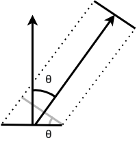
The most important density of power is radiance. Radiance is the density of power with respect to both solid angle (of the unit hemisphere surrounding a point) and projected area (surrounding a point on a surface). Thus, power is computed as

\[\Phi = \int_A \int_{\Omega} L(p, \omega) \cos \theta ~d\omega~dA,\]

where \(\theta\) again represents the incident angle. We must multiply by a factor of \(\cos \theta\) to convert area to projected area (\(A^{\perp}\) above). Thus, radiance is defined with respect to a surface perpendicular to the incident direction and not with respect to the surface containing the point \(p\).

Thus, irradiance is a density of radiance, such that

\[E(p) = \int_{\Omega} L(p,\omega) \cos \theta ~d\omega.\]

Thus, we will sometimes write

\[E(p,\omega) = L(p,\omega) \cos \theta.\]

The bidirectional reflectance distribution function (BRDF) is one of the most important radiometric concepts for rendering. It provides a means for describing the reflection of light from a surface. The BRDF determines many of the characteristics of the appearance of surfaces when rendered. The BRDF is essentially a ratio which describes the proportion of reflected light. It is typically denoted

\[f_r(p,\omega_o,\omega_i),\]

where \(p\) is a point on the surface, \(\omega_o\) is the outgoing direction and \(\omega_i\) is the incoming direction, as in Figure 16.

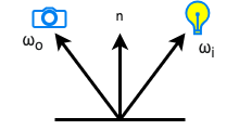
Note that the vectors \(\omega_o\) and \(\omega_i\) both originate from the point \(p\); this views them as vectors in a vector space whose origin is \(p\). Otherwise, the vectors would not be comparable.

We will use the notation \(L_o(p,\omega_o,\omega_i)\) to indicate the density of radiance with respect to incident directions (where \(H^2\) is the upper unit hemisphere):

\[L_o(p,\omega_o) = \int_{H^2}L_o(p,\omega_o,\omega_i)~d\omega_i.\]

More specifically, the BRDF indicates the ratio of exitant radiance to irradiance:

\[f_r(p,\omega_o,\omega_i) = \frac{L_o(p,\omega_o, \omega_i)}{E(p,\omega_i)} = \frac{L_o(p,\omega_o, \omega_i)}{L_i(p,\omega_i)\cos \theta_i}.\]

Thus, if \(L_i(p,\omega_i)\) is the incident radiance at \(\omega_i\), then \(L_o(p, \omega_o, \omega_i) = f_r(p,\omega_o,\omega_i)L_i(p,\omega_i)\cos \theta_i\) gives the exitant radiance at \(\omega_o\) due to \(\omega_i\). Thus, the total exitant radiance can be determined by integrating over all incident directions (where \(H^2\) is the upper unit hemisphere):

\[L_o(p,\omega_o) = \int_{H^2} f_r(p,\omega_o,\omega_i)L_i(p,\omega_i)~\cos \theta_i ~d\omega_i.\]

Physically based BRDFs are subject to additional constraints:

1. Reciprocity: \(f_r(p,\omega_o,\omega_i) = f_r(p,\omega_i,\omega_o)\) for all directions \(\omega_i,\omega_o\) and points \(p\). This expresses a symmetry in the reflectance.
2. Energy conservation: the total reflection over the hemisphere is less than or equal to the energy of incident light:

\[\int_H f_r(p,\omega_o,\omega_i)\cos \theta_i ~d\omega_i \leq 1.\]

The bidirectional transmittance distribution function (BTDF) is very similar to the BRDF, except that the directions \(\omega_o\) and \(\omega_i\) lie in different hemispheres around the point \(p\), as in Figure 17.

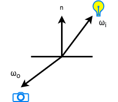
The BTDF is usually denoted

\[f_t(p,\omega_o,\omega_i).\]

Physically based BTDFs do not necessarily obey reciprocity, but they do obey energy conservation.

The BRDF and BTDF are often combined into a single function called the bidirectional scattering distribution function (BSDF). The BSDF is denoted

\[f(p,\omega_o,\omega_i).\]

Thus, we've arrived at one of the fundamental equations of rendering: the scattering equation, which is

\[L_o(p,\omega_o) = \int_{S^2} f(p,\omega_o,\omega_i)\lvert \cos \theta_i \rvert ~d\omega_i.\]

The \(\cos \theta_i\) factor is amended to an absolute value to account for the fact that surface normals might lie in a different hemisphere than the respective directions.

The scattering equation will form the basis for the light transport equation (also called the rendering equation) which will be discussed subsequently.

Scattering Functions

Now that we've described the general theory of scattering functions, let's consider a few examples.

Diffuse Reflection

The simplest BRDF represents perfectly diffuse reflection which scatters incident light equally in all directions. Thus, the total reflectance is a constant \(R\).

\[\int_{H^2(n)}f_r(p,\omega_o,\omega_i)\cos \theta_i ~d\omega_i = R\]

However, in order to obey the conservation of energy, it must be the case that \(R \in [0, 1].\) Then, since

\begin{align}\int_{H^2(n)}\cos \theta_i ~d\omega_i &= \int_0^{2\pi} \int_0^{\pi/2} \cos \theta_i \sin \theta_i ~d\theta_i ~d\varphi \\&= \int_0^{2\pi} (\frac{\sin^2(\frac{\pi}{2})}{2} - \frac{\sin^2(0)}{2}) ~d\varphi \\&= \int_0^{2\pi} \frac{1}{2} ~d\varphi \\&= \frac{2\pi}{2} - 0 \\&= \pi,\end{align}

if we normalize by a factor of \(1/\pi\), then

\begin{align}\int_{H^2(n)}f_r(p,\omega_o,\omega_i)\cos \theta_i ~d\omega_i &= \int_{H^2(n)}\frac{R}{\pi}\cos \theta_i ~d\omega_i \\&= \frac{R}{\pi} \int_{H^2(n)}\cos \theta_i ~d\omega_i \\&= \frac{R}{\pi} \cdot \pi \\&= R.\end{align}

Thus, the BRDF for perfectly diffuse reflection is

\[f_r(p,\omega_o,\omega_i) = \frac{R}{\pi}.\]

Specular Reflection

Another simple BRDF is the BRDF for perfect specular reflection ("mirror" reflection) which scatters incident light in exactly one direction, namely, the reflection \(\omega_r\) across the surface normal. This BRDF is represented by a distribution rather than a function. We want the scattering equation to "integrate" to \(1\) (i.e. we want the action of the distribution in the context of the scattering equation to yield \(1\)), since a perfect specular BRDF reflects all of the incident light:

\[\int_{H^2(n)}f_r(p, \omega_o, \omega_i) \cos \theta_i ~d\omega_i = 1.\]

As a first attempt, we might define the BRDF as

\[f_r(p,\omega_o,\omega_i) = \delta_{\omega_r},\]

where \(\omega_r\) is the reflection of \(\omega_o\) across the surface normal \(n\) at the point \(p\). However, when computing the action of this distribution, we discover the following:

\begin{align}\int_{H^2(n)}f_r(p, \omega_o, \omega_i) \cos \theta_i ~d\omega_i &=\int_{H^2(n)}\delta_{\omega_r} \cos \theta_i ~d\omega_i \\&= \delta_{\omega_r}[\cos \theta] \\&= \cos \theta_r.\end{align}

Thus, it is not equal to \(1\) as desired. Instead, we define the BRDF as

\[f_r(p,\omega_o,\omega_i) = \frac{\delta_{\omega_r}}{\cos \theta_r},\]

which is the distribution which acts on a test function \(\psi\) as follows:

\[ \frac{\delta_{\omega_r}}{\cos \theta_r}[\psi] = \frac{\psi(\omega_r)}{\cos \theta_r}.\]

Thus, the integral is

\begin{align}\int_{H^2(n)}f_r(p, \omega_o, \omega_i) \cos \theta_i ~d\omega_i &=\int_{H^2(n)}\frac{\delta_{\omega_r}}{\cos \theta_r} \cos \theta_i ~d\omega_i \\&= \frac{\cos \theta_r}{\cos \theta_r} \\&= 1.\end{align}

Dielectric BSDF

Given incident direction \((\theta_i, \varphi_i)\) as in Figure X, the reflected direction, expressed using pairs of angles (as in Figure 18), is

\[\theta_r = \theta_i,~ \varphi_r = \varphi_i + \pi.\]

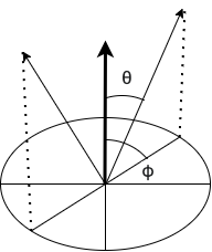
It is often more convenient to express this relationship using vectors. Each vector can be decomposed into its components within the reflection plane, one parallel and one perpendicular component, as in Figure 19.

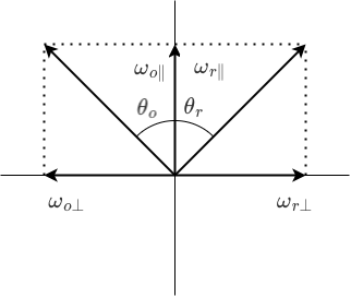
Thus, \(\omega_o = \omega_{o\perp} + \omega_{0\parallel}\). Futhermore, \(\omega_{o\parallel} = (n \cdot \omega_o)n\) and \(\omega_{o\perp} = \omega_o - \omega_{o\parallel}\). Likewise, \(\omega_r = \omega_{r\perp} + \omega_{r\parallel}\). We can then compute

\begin{align}\omega_r &= \omega_{r\perp} + \omega_{r\parallel} \\&= -\omega_{o\perp} + \omega_{o\parallel} \\&= -(\omega_o - \omega_{o\parallel}) + (n \cdot \omega_o)n \\&=-(\omega_o - (n \cdot \omega_o)n) + (n \cdot \omega_o)n \\&= -\omega_o + 2(n \cdot \omega_o)n.\end{align}

Likewise, given incident direction \((\theta_i, \varphi_i)\), Snell's Law states that the transmitted (refracted) direction \((\theta_t,\varphi_t)\) satisfies the following relationships:

\[\eta_i \sin \theta_i = \eta_t \sin \theta_t, ~\varphi_i = \varphi_t,\]

where \(\eta_i\) and \(\eta_t\) represent the index of refraction of the exterior and interior of the surface, respectively. This can be expressed in terms of the relative index of refraction \(\eta\) defined as follows:

\[\eta = \frac{\eta_t}{\eta_i}.\]

Thus, it follows that

\[\sin \theta_i = \eta \sin \theta_t.\]

Next, consider the vectorial description of refraction as in Figure 20.

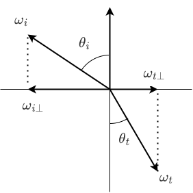
Since \(\lVert \omega_t \rVert \sin \theta_t = \lVert \omega_{t\perp}\rVert\), it follows that \(\lVert \omega_t \rVert (1/\eta) \sin \theta_i = \lVert \omega_{t\perp}\rVert\). If we adopt the convention that \(\omega_i\) and \(\omega_t\) are normalized (have unit length), then \((1/\eta) \sin \theta_i = \lVert \omega_{t\perp}\rVert\). Since \(\sin \theta_i = \lVert \omega_{i\perp}\rVert/\lVert \omega_i \rVert\), it follows that \(\sin \theta_i = \lVert \omega_{i\perp}\rVert\). Then, substituting, we obtain \((1/\eta) \lVert \omega_{i\perp}\rVert = \lVert \omega_{t\perp}\rVert\). It thus follows that

\[\omega_{t\perp} = \frac{-\omega_{i\perp}}{\eta}.\]

Then, since \(\omega_{i\perp} = \omega_i - \omega_{i\parallel}\) and \(\omega_{i\parallel} = (\omega_i \cdot n)n\), it follows that

\[\omega_{t\perp} = \frac{-(\omega_i - (\omega_i \cdot n)n)}{\eta}.\]

Since \(\omega_{t\parallel}\) points in the direction \(-n\), it follows that

\[\omega_{t\parallel} = -(\omega_t \cdot n)n.\]

Thus, finally, we have that

\[\omega_t = \omega_{t\perp} + \omega_{t\parallel} = \frac{-\omega_i}{\eta} + \left[\frac{\omega_i \cdot n}{\eta} - \omega_t \cdot n\right]n.\]

The Fresnel equations indicate the amount of transmitted light:

\[r_{\parallel} = \frac{\eta_t \cos \theta_i - \eta_i \cos \theta_t}{\eta_t \cos \theta_t + \eta_i \cos \theta_t},\]

\[r_{\perp} = \frac{\eta_i \cos \theta_i - \eta_t \cos \theta_t}{\eta_i \cos \theta_i + \eta_i \cos \theta_t}.\]

Using the relative index of refraction \(\eta\), this is equivalent to

\[r_{\parallel} = \frac{\eta \cos \theta_i - \cos \theta_t}{\eta \cos \theta_t + \cos \theta_t},\]

\[r_{\perp} = \frac{\cos \theta_i - \eta \cos \theta_t}{\cos \theta_i + \eta \cos \theta_t}.\]

The Fresnel reflectance is then given by

\[F_r = \frac{r_{\parallel} + r_{\perp}}{2}.\]

We require a BRDF such that the reflectance function yields precisely the proportion of the incident radiance reflected according to the Fresnel reflectance, namely:

\[\int_{H^2(n)} f_r(p,\omega_o,\omega_i)L_i(\omega_i)\lvert\cos \theta_i\rvert~d\omega_i = F_r(\omega_r)L_i(\omega_i).\]

Just as before, we must compensate for the \(\lvert \cos \theta_i \rvert\) term; we define the BRDF as follows:

\[f_r(p,\omega_o,\omega_i) = \frac{F_r(\omega_r)}{\lvert \cos \theta_r \rvert} \delta_{\omega_r}.\]

We then compute

\begin{align}\int_{H^2(n)} f_r(p,\omega_o,\omega_i)L_i(\omega_i)\lvert\cos \theta_i\rvert~d\omega_i &= \int_{H^2(n)} \frac{F_r(\omega_r)}{\lvert \cos \theta_r \rvert} \delta_{\omega_r}L_i(\omega_i)\lvert\cos \theta_i\rvert~d\omega_i \\&= \frac{F_r(\omega_r)}{\lvert \cos \theta_r\rvert} L_i(\omega_r)\lvert\cos \theta_r \rvert \\& = F_r(\omega_r)L_i(\omega_r).\end{align}

All BRDFs defined above are defined with respect to solid angle. When a BRDF is defined using a distribution, it should not be converted from solid angle to area; the action of the distribution computes the final result, and it does not need to be adjusted. The conversion from solid angle to area is only within an integrand; it does not apply to the final result.

Color

Each of the radiometric measures defined previously were defined irrespective of their variation with respect to the wavelength of light. Each has a corresponding spectral variant which is a density with respect to wavelength. For instance, spectral radiance \(L_{\lambda}\) is the density of radiance with respect to wavelength:

\[L(p, \omega) = \int_{\lambda_1}^{\lambda_2} L_{\lambda}(p, \omega, \lambda) ~d\lambda.\]

Thus, integrating spectral radiance over a range of wavelengths yields radiance. In general, a spectral distribution is a density of some radiometric measure with respect to wavelength.

Spectral distributions are radiometric concepts defined independently from human perception of color. However, we are ultimately interested in producing images which can be perceived by human subjects. The tristimulus theory of color perception maintains that three scalar values \((v_1,v_2,v_3)\) are sufficient to represent any (visible) spectral distribution for human observers. This theory is based on the biological fact that there are three types of receptor cones in the human eye, and has been tested in many experiments. Such tests have resulted in empirically determined spectral matching functions. A set of spectral matching functions consists of three functions \(m_1(\lambda), m_2(\lambda), m_2(\lambda)\) which, when integrated against a spectral distribution \(S(\lambda)\) as follows, yields the respective tristimulus value:

\[v_i = \int_{\lambda_1}^{\lambda_2} S(\lambda) m_i(\lambda) ~d\lambda.\]

A set of matching functions defines a color space, which is a \(3\)-dimensional real vector space consisting of vectors of tristimulus values.

Although color spaces enjoy certain nice properties, they do not inherit all of the properties enjoyed by spectral distributions (for instance, they do not preserve products of spectral distributions). For this reason, many renderers choose to work directly with spectral distributions, and not within any color space; color is determined only after rendering of spectra is complete.

In the prototype Rust implementation, spectral distributions were not used. Instead, the renderer computes within a linear RGB color space directly. However, in a more fully-featured renderer, it would be preferable to use spectral distributions.

Lights

Each scene requires at least one source of light to illuminate the objects in the scene. One simple example of a light is a diffuse area light. A diffuse area light is a light with a given shape (e.g. a sphere) whose emission is uniformly distributed over the surface of the shape, that is, at each point there is a uniform directional distribution of light. Such lights are therefore relatively easy to implement.

The Light Transport Equation

The light transport equation (LTE) (or rendering equation) is based on the principle of energy balance.

The LTE implies that the exitant radiance must be the sum of the incident radiance scattered from a surface and the emitted radiance on the surface. This principle yields the light transport equation:

\[L_o(p,\omega_o) = L_e(p,\omega_o) + \int_{S^2}f(p,\omega_o,\omega_i)L_i(p,\omega_i)\lvert cos \theta_i \rvert d\omega_i.\]

This equation is based directly on the scattering equation. The ray casting function \(t(p,\omega)\) computes the closest point \(p\) on any surface in a scene intersected by a ray with origin \(p\) and direction \(\omega\). If the scene is open and no point is intersected by the ray, this function returns a special value indicating that there is no intersection. All functions composed with the ray casting function implicitly evaluate to \(0\) for this special value. The ray casting function can only be defined implicitly (that is, numerically, in source code). Thus, it is left abstract.

The incoming radiance \(L_o\) can then be expressed in terms of the outgoing radiance:

\[L_i(p,\omega) = L_o(t(p,\omega),-\omega).\]

This allows us to rewrite the LTE using only outgoing radiance:

\[L_o(p,\omega_o) = L_e(p,\omega_o) + \int_{S^2}f(p,\omega_o,\omega_i)L_o(t(p,\omega_i),-\omega_i)\lvert cos \theta_i \rvert d\omega_i.\]

The LTE then becomes a recursive equation where the outgoing radiance at some point and direction is expressed in terms of the outgoing radiance at related points and directions. Thus, there is only a single quantity which must be calculated. By expanding this recursive equation, we can arrive at a non-recursive equation which is more amenable for certain purposes.

Thus, we want to simplify the LTE in 3 ways:

1. We want to make the effect of the ray casting function explicit.
2. We want to eliminate the recursion by expanding it to an iterative expression.
3. We want the integral to be expressed with respect to area rather than with respect to direction. This will allow us to express the integral more uniformly (in terms of points on surfaces, rather than a combination of points and directions).

The next step is to express the integral with respect to area. It will be very useful to introduce new notation.

First, we define

\[L_o(p' \rightarrow p) = L_o(p,\omega)\]

where

\[\omega = \frac{p - p'}{\lVert p - p' \rVert}\]

Likewise, for the BRDF, we define

\[f(p'' \rightarrow p' \rightarrow p) = f(p',\omega_o,\omega_i),\]

where, again,

\[\omega_o = \frac{p - p'}{\lVert p - p' \rVert}\]

and

\[\omega_i = \frac{p' - p''}{\lVert p' - p'' \rVert}.\]

We also must apply the conversion term for converting from solid angle to area. It is convenient to group the factor \(\lvert \cos \theta \rvert\) from the LTE together with this conversion term into a geometry term defined as

\[G(p \leftrightarrow p') = V(p \leftrightarrow p')\frac{\lvert \cos \theta \rvert \lvert \cos \theta' \vert}{\lVert p - p' \rVert^2},\]

where the visibility term \(V(p \leftrightarrow p')\) is \(1\) if the points are mutually visible (rays can be cast between them without intersecting any other surface) and \(0\) otherwise. In practice, since we evaluate integrals numerically and only sample points that are mutually visible, we do not need to account for the visibility term explicitly.

The surface form of the LTE can then be expressed as follows:

\[L_o(p' \rightarrow p) = L_e(p' \rightarrow p) + \int_A f(p'' \rightarrow p' \rightarrow p)L_o(p'' \rightarrow p')G(p'' \leftrightarrow p')dA(p'').\]

The domain of integration \(A\) represents the union of all surfaces in the scene. The notation \(dA(p)\) simply indicates which point corresponds to the measure \(dA\).

Next, we will expand the surface for of the LTE in order to eliminate the recursion.

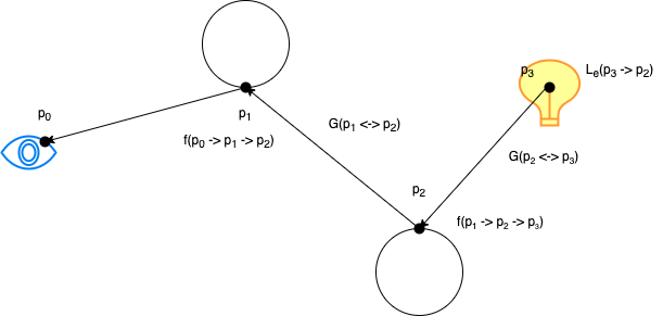
We will first consider a single expansion (and hence a path consisting of 4 points, as in Figure 21). The LTE indicates that

\[L_o(p_1 \rightarrow p_0) = L_e(p_1 \rightarrow p_0) + \int_A f(p_2 \rightarrow p_1 \rightarrow p_0)L_o(p_2 \rightarrow p_1)G(p_2 \leftrightarrow p_1)dA(p_2).\]

Thus, we also have that

\[L_o(p_2 \rightarrow p_1) = L_e(p_2 \rightarrow p_1) + \int_A f(p_3\rightarrow p_2 \rightarrow p_1)L_o(p_3 \rightarrow p_2)G(p_3 \leftrightarrow p_2)dA(p_3).\]

Since \(p_3\) is on a light source, the LTE reduces to \(L_o(p_3 \rightarrow p_2) = L_3(p_3 \rightarrow p_2)\) since the light source only emits radiance (we do no regard any reflectance on the light source). Thus, substituting the expression for \(L_o(p_2 \rightarrow p_1)\) into the expression for \(L_o(p_2 \rightarrow p_1)\), we obtain

\begin{align}L(p_1 \leftrightarrow p_0) &= L_e(p_1 \rightarrow p_0) + \int_A f(p_2 \rightarrow p_1 \rightarrow p_0)L_o(p_2 \rightarrow p_1)G(p_2 \leftrightarrow p_1)dA(p_2) \\&= L_e(p_1 \rightarrow p_0) + \int_A f(p_2 \rightarrow p_1 \rightarrow p_0)\left[L_e(p_2 \rightarrow p_1) + \int_A f(p_3\rightarrow p_2 \rightarrow p_1)L_e(p_3 \rightarrow p_2)G(p_3 \leftrightarrow p_2)dA(p_3)\right]G(p_2 \leftrightarrow p_1)dA(p_2) \\&= L_e(p_1 \rightarrow p_0) + \int_A L_e(p_2 \rightarrow p_1) f(p_2 \rightarrow p_1 \rightarrow p_0)G(p_2 \leftrightarrow p_1)dA(p_2) + \int_A \int_A L_e(p_3 \rightarrow p_2) f(p_3\rightarrow p_2 \rightarrow p_1)G(p_3 \leftrightarrow p_2) f(p_2 \rightarrow p_1 \rightarrow p_0) G(p_2 \leftrightarrow p_1) dA(p_3)dA(p_2).\end{align}

Next, we will introduce some useful terminology. A path \(\bar{p}_n\) is an ordered tuple of \(n+1\) points (called vertices) with indices from \(0\) to \(n\), i.e. \(\bar{p}_n = (p_0, \dots, p_n)\). The throughput of a path is defined as

\[T(\bar{p}_n) = L(p_n \rightarrow p_{n-1})\prod_{i=1}^{n-1}f(p_{i+1} \rightarrow p_i \rightarrow p_{i-1})G(p_{i+1} \leftrightarrow p_i).\]

Note that some authors do not include the term \(L(p_n \rightarrow p_{n-1})\) as part of the throughput. We can then define the expression

\[P(\bar{p}_n) = \int_{A^{n-1}}T(\bar{p}_n)dA(p_n)\dots dA(p_2),\]

where \(A^{n-1}\) denotes the \((n-1)\)-times iterated integral over \(A\).

We can then rewrite the expansion above as

\[L(p_1 \rightarrow p_o) = L_e(p_1 \rightarrow p_0) + \int_A T(\bar{p}_2) dA(p_2) + \int_A \int_A T(\bar{p}_3) dA(p_3)dA(p_2),\]

or as

\[L(p_1 \rightarrow p_o) = \sum_{i=1}^3 P(\bar{p}_i).\]

Since this pattern continues indefinitely, we now have an iterative form of the LTE which we can us to approximate the LTE to an arbitrary degree of accuracy (i.e. up to a given path length \(n\)); once a path is terminated at a light source, the expression for \(P(\bar{p}_n)\) is simply \(L_e\), the emitted radiance from the light source.

The Measurement Equation

The light transport equation permits us to define the radiance \(L(p_1 \rightarrow p_0)\) transmitted from a point \(p_1\) to a point \(p_0\) lying on the camera plane. However, the radiometric quantity that we actually measure is radiant power. Thus, we need to define an equation that computes the radiant power \(I_j\) at each pixel \(j\) on the camera plane. Since radiance is a density of power, we integrate as follows to compute power:

\[I_j = \int_{A_{film}} \int_{S^2} W_e^{(j)}(p_0,\omega) L_i(p_o, \omega) ~\lvert \cos \theta \rvert ~d\omega ~dA(p_0).\]

The term \(W_e^{(j)}\) is called importance and calibrates the camera's sensitivity at each pixel; it will be explained shortly.

Rewriting this as an integral over area, we obtain

\[I_j = \int_{A_{film}} \int_A W_e^{(j)}(p_0 \rightarrow p_1) L(p_1 \rightarrow p_0) ~G(p_1 \leftrightarrow p_0) ~dA(p_1) ~dA(p_0).\]

If we expand this equation, we obtain the following:

\begin{align}I_j &= \int_{A_{film}} \int_A W_e^{(j)}(p_0 \rightarrow p_1) L(p_1 \rightarrow p_0) ~G(p_1 \leftrightarrow p_0) ~dA(p_1) ~dA(p_0) \\&= \int_{A_{film}} \int_A W_e^{(j)}(p_0 \rightarrow p_1) \left(\sum_i P(\bar{p}_i)\right)~G(p_1 \leftrightarrow p_0) ~dA(p_1) ~dA(p_0) \\&= \sum_i \int_{A_{film}} \int_A W_e^{(j)}(p_0 \rightarrow p_1) P(\bar{p}_i)~G(p_1 \leftrightarrow p_0) ~dA(p_1) ~dA(p_0) \\&= \sum_i \int_{A_{film}} \int_{A^{i+1}} W_e^{(j)}(p_0 \rightarrow p_1) T(\bar{p}) ~G(p_1 \leftrightarrow p_0) ~dA(p_i)\dots dA(p_0).\end{align}

If we define the extended throughput \(T^+(\bar{p})\) as

\[T^+(\bar{p}_n) = W_e^{(j)}(p_0 \rightarrow p_1) T(\bar{p}_n) ~G(p_1 \leftrightarrow p_0),\]

then we can rewrite the equation as

\[I_j = \sum_i \int_{A_{film}} \int_{A^{i+1}} T^+(\bar{p}_i) ~dA(p_i)\dots dA(p_0).\]

If we consider the irradiance at the pinhole expressed in terms of incident radiance, we get

\[E(p) = \int_{A_{\text{film}}}L(p,\omega)\cos \theta~d\omega.\]

If we convert to an integral over film area, we get

\[E(p) = \int_{A_{\text{film}}}L(p,\omega) \frac{\cos \theta \cos \theta'}{\lVert p - p' \rVert}~dA(p').\]

Noting that \(\theta = \theta'\), if we write \(d = \lVert p - p' \rVert\) and the camera distance as \(z = d/\cos \theta\), then we obtain

\[E(p) = \int_{A_{\text{film}}}L(p,\omega) \frac{\cos \theta \cos \theta}{\left(\frac{z}{\cos \theta}\right)^2}~dA(p') = \int_{A_{\text{film}}}L(p,\omega) \frac{\cos^4\theta}{z^2}~dA(p').\]

We then introduce the importance function \(W_e(p,\omega)\) and require it to be normalized such that

\[\int_{A_{\text{film}}}W_e(p \rightarrow p')G(p \leftrightarrow p')~dA(p') = 1.\]

If the define \(W_e\) as the reciprocal of the geometric term \(\frac{\cos^4\theta}{z^2}\), i.e. as \(\frac{z^2}{\cos^4\theta}\) and divide by the area \(A\) of the film in order to normalize, we obtain

\[W_e(p \rightarrow p') = \frac{z^2}{A \cos^4\theta},\]

and thus

\[\int_{A_{\text{film}}}W_e(p \rightarrow p')G(p \leftrightarrow p')~dA(p') = \int_{A_{\text{film}}} \frac{1}{A} = 1.\]

The importance function thus corrects for the decrease in irradiance; this phenomenon is called vignetting. Many real cameras will correct for vignetting.

The measurement equation also accounts for the filter function (see image reconstruction below) and the fact that only certain incident directions are actually measured (since only directions passing from the camera origin through the film plane are measured, which is automatically handled in the ray tracing algorithm since only such directions are considered).

Sampling

Importance Sampling

Importance sampling is a technique for reducing the variance of a Monte Carlo estimator. Recall that the Monte Carlo estimator is

\[E[f] = \sum_{x \in X}\frac{f(x)}{p(x)}.\]

If a PDF \(p\) is chosen which is proportional to \(f\), i.e. \(p(x) = cf(x)\) for some \(c\) (here we will assume that \(f(x) \ge 0\), then, since the PDF is subject to the normalization constraint

\[\int p(x)~dx = 1,\]

it follows that

\[\int p(x)~dx = \int cf(x)~dx = 1,\]

and thus

\[c = \frac{1}{\int f(x)~dx}.\]

Then, the ratio

\[\frac{f(x)}{p(x)} = \frac{f(x)}{c(fx)} = \frac{1}{c} = \int f(x)~dx.\]

Thus, the variance is \(0\). Of course, in this case, Monte Carlo integration would be unnecessary since we can already compute the integral, but it demonstrates that a PDF that is proportional to the function being estimated will reduce variance.

In practice, we use importance sampling when sampling lights, BSDFs, etc. during path tracing.

Multiple Importance Sampling

Often, we have multiple sampling strategies at our disposal. The question then arise of how to compute a Monte Carlo estimate, i.e. which respective sampling distribution to use.

The technique of multiple importance sampling used a weighted combination as an estimate. For instance, given two random variables \(X\) and \(Y\) drawn from distributions \(p_a\) and \(p_b\), the MIS estimate is

\[w_a(X)\frac{f(X)}{p_a(X)} + w_b(Y)\frac{f(Y)}{p_b(Y)}.\]

The weights are subject to the constraint that the estimator must remain unbiased (i.e. the expected value of the resulting Monte Carlo estimator must still be the integral being estimated).

Thus, given \(n\) such distributions \(p_i\) with \(n_i\) samples from each and random variables \(X_{i,j}\) sampled from \(p_i\) with \(1 \leq j \leq n_i\), we obtain

\[E[f] = \sum_{i=1}^n\frac{1}{n_i}\sum_{j=1}^{n_i}\frac{w_i(X_{i,j})}{p_i(X_{i,j})}.\]

A common choice for an MIS weighting scheme is the balance heuristic, which is

\[w_i(X) = \frac{n_i p_i(X)}{\sum_{j=1}^{n_i}n_j p_j(X)}.\]

Metropolis Sampling

A Markov chain can be conceived as a state machine with probabilistic transitions, as in Figure 22.

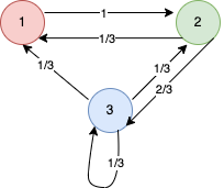
In order to describe Markov chains, it is useful to introduce some terminology. A probability space \((\Omega, \mathcal{E}, P)\) consists of the following data:

• A sample space \(\Omega\) (which is any set, whose elements are called outcomes)
• A set of events \(\mathcal{E}\); each event is a subset of the sample space (i.e. it is a set of one or more outcomes). The set \(\mathcal{E}\) must be a \(\sigma\)-algebra, i.e. \(\Omega \in \mathcal{E}\) and \(\mathcal{E}\) is closed under complements and finite unions and intersections.
• A probability measure \(P : \mathcal{E} \rightarrow [0,1]\) which assigns a probability to each event. It must satisfy the properties \(P(\mathcal{\Omega}) = 1\) and \(\sum_{e \in E}P(e) = P(\cup E)\) for each countable set of events \(E \subseteq \mathcal{E}\).

A random variable is a function \(X : \Omega \rightarrow V\) that assigns to each outcome a particular value in some measurable set \(V\) (a measurable space \((M,\mathcal{F})\) consists of a set \(M\) and a \(\sigma\)-algebra \(\mathcal{F}\) on \(M\), and a measurable set is an element \(V \in \mathcal{F}\)). It must satisfy the property \(X^{-1}(S) \in \mathcal{E}\) for all \(S \subseteq V\).

The probability that a random variable \(X\) assumes a value in a measurable set \(S \subseteq V\) is given by is probability distribution

\[P(X \in S) = P(X^{-1}(S)) = P(\{\omega \in \Omega \mid X(\omega) \in S\}).\]

A random variable is discrete if it takes values in countable set \(V\). Otherwise, if \(V\) is uncountably infinite, the random variable is called continuous.

For discrete random variables, we also often write

\[P(X = s) = P(X \in \{s\}) = P(\{\omega \in \Omega \mid X(\omega) = s\}).\]

A probability mass function for a discrete random variable \(X\) is a function \(p_X : V \rightarrow [0,1]\) such that

\[p_X(v) = P(X = v).\]

However, for continuous random variables, it does not make sense to define such a function (the probability measure for a singleton set \(\{v\}\) is \(0\)). Instead, for absolutely continuous real-valued random variables \(X : \Omega \rightarrow \mathbb{R}\), the probability density function (PDF) is the function \(f_X\) such that

\[P(a \leq v \leq b) = \int_a^b f_X(v)~dv.\]

In the case that the random variable \(X\) is real-valued (i.e. \(X : \Omega \rightarrow \mathbb{R}\)), the cumulative distribution function (CDF) is defined as

\[F_X(v) = P(X \leq v) = P(\{\omega \in \Omega \mid X(\omega) \leq v\}).\]

When the CDF is invertible, the quantile function or inverse CDF can map a number in the range \([0, 1]\) to its corresponding threshold value:

\[F_X^{-1}(p) = v, P(X \leq v) = p.\]

This is useful for sampling the CDF, for instance; a uniformly distributed random number in the range \([0, 1]\) can be generated, and the inverse CDF will map it to a value.

Although random variables are important for theoretical purposes, we are generally interested in their distributions, so the distribution is defined and the random variable and probability space are suppressed. The distributions are generally expressed via a CDF or PDF.

A Markov chain consists of the following data:

• A state space \(\mathcal{S}\) which is a measurable set whose elements are called states
• A probability space \((\Omega, \mathcal{E}, P)\)
• A sequence of random variables \((X_i : \Omega \rightarrow \mathcal{S})\),
• A probability distribution \(\pi_0\) for \(X_0\) called the initial distribution (which indicates the relative likelihood of beginning in a particular state)
• A transition function \(P(s_i \mid s_j) : \mathcal{S} \times \mathcal{S} \rightarrow [0,1]\) (which indicates the conditional probability of a transition from \(s_j\) to \(s_i\))

Example

Consider the Markov chain depicted in Figure 22. Its sample space is thus the set \(\{1,2,3\}\). Suppose that we choose samples using a uniformly distributed pseudo-random number generator (PRNG) on a computer, which generates numbers in the range \([0,1]\). Suppose that the initial distribution \(\pi_0\) is defined so that \(\pi_0(1) = 1/2\), \(\pi_0(2) = 1/4\), and \(\pi_0(3) = 1/4\) (note that specifying the values for each state completely determines its values on all subsets of states). We can define the inverse cumulative distribution corresponding to \(\pi_0\):

\[F^{-1}_0(x) = \begin{cases}1 & \text{if} ~ 0 \leq x \leq \frac{1}{2}, \\ 2 & \text{if} ~ \frac{1}{2} \lt x \leq \frac{3}{4}, \\ 3 & \text{if} ~ \frac{3}{4} \lt x \leq 1.\end{cases}\]

Next, we define a sequence of random numbers \((x_i)\). In this example, they will be generated by the PRNG. Suppose that \(x_0 = 0.84\). Then \(F^{-1}_0(s_0) = 3\), so the first state is state \(3\).

Next, another distribution \(\pi_1\) can be constructed such that

\[\pi_1(s) = \sum_{s' \in \mathcal{S}}\pi_0(s')P(s \mid s').\]

Thus, we can then define the next inverse CDF \(F^{-1}_1\) as

\[F^{-1}_1(s) = \begin{cases}1 & \text{if} ~ 0 \leq x \leq \frac{1}{6}, \\ 2 & \text{if} ~ \frac{1}{6} \lt x \leq \frac{7}{12}, \\ 3 & \text{if} ~ \frac{7}{12} \lt x \leq 1.\end{cases}\]

We can continue indefinitely and define the distribution \(\pi_t\) at time \(t\) recursively using the Law of Total Probability as follows:

\[\pi_{t+1}(s_j) = \sum_{i=1}^n \pi_t(s_i)P(s_j \mid s_i).\]

A stationary distribution (or equilibrium distribution) is a distribution \(\pi\) such that

\[\pi(s_j) = \sum_{i = 1}^n \pi(s_i)P(s_j \mid s_i).\]

In other words, a stationary distribution is one which remains constant once achieved.

Under certain circumstances, a Markov chain will possess a stationary distribution. A sufficient condition is that the chain exhibits detailed balance, which means that there is a symmetry in transitions:

\[P(s' \mid s)P(s) = P(s \mid s')P(s').\]

The stationary distribution will be unique if the Markov chain is ergodic (basically, it is possible to arrive at every state with non-zero probability; formally, the chain is aperiodic and positive recurrent).

The Metropolis-Hastings Algorithm

The Metropolis sampling algorithm designs a Markov chain such that the stationary distribution \(\pi\) is equal to some desired distribution \(P\).

First, the condition of detailed balance is required, which is re-written in the following form:

\[\frac{P(s' \mid s)}{P(s \mid s')} = \frac{P(s')}{P(s)}.\]

The transition distribution is then decomposed into two components: the proposal distribution \(g(s' \mid s)\) and the acceptance distribution \(a(s' \mid s)\) (which describe the probability of proposing a given transition and accepting a given transition, respectively). Thus

\[P(s' \mid s) = g(s' \mid s)a(s' \mid s).\]

Substituting into the equation for detailed balance, we obtain

\[\frac{g(s' \mid s)a(s' \mid s)}{g(s \mid s')a(s \mid s')} = \frac{P(s')}{P(s)},\]

which we can rewrite as

\[\frac{a(s' \mid s)}{a(s \mid s')} = \frac{P(s')g(s \mid s')}{P(s)g(s' \mid s)}.\]

Thus, our object is to choose an acceptance distribution which fulfills the requirement of detailed balance, and thus satisfies this equation. The most common choice is the following:

\[a(s' \mid s) = \mathrm{min}\left(1, \frac{P(s')g(s \mid s')}{P(s)g(s' \mid s)}\right).\]

Either \(a(s' | s)\) or \(a(s | s')\) will be \(1\) and the equation will then hold by construction.

Note that, if the transition probabilities are symmetric, i.e. \(g(s' \mid s) = g(s \mid s')\), then the acceptable probability becomes simply

\[a(s' \mid s) = \mathrm{min}\left(1, \frac{P(s')}{P(s)}\right).\]

This yields the following algorithm, called the Metropolis-Hastings Algorithm:

1. Choose an initial state \(s_0\). Set \(i=0\).
2. Generate a random candidate state \(s'\) according to \(g(s' \mid s_i)\).
3. Calculate the acceptance probability \(a(s' \mid s_i)\).
4. Accept or reject:
   1. Generate a random number \(u\) in the range \([0,1]\).
   2. If \(u \leq a(s' \mid s_i)\), then accept: \(s_{i+1} = s'\).
   3. If \(u \gt a(s' \mid s_i)\), then reject: \(s_{i+1} = s_i\).
5. Continue to step 2 with \(i = i + 1\).

The application of the Metropolis-Hastings sampling algorithm to Monte Carlo integration is an example of a Markov Chain Monte Carlo (MCMC) technique. In particular, the distribution that we want to sample when integrating a function is the function's own distribution, namely

\[p(x) = \frac{f(x)}{\int f(x) ~dx}.\]

However, we do not know this distribution; indeed, our goal is to calculate the integral of \(f\) in the first place. If we know a function \(I\) which is proportional to \(f\) and we know its integral, then we can generate samples distributed according to \(I\)'s distribution, namely

\[p(x) = \frac{I(x)}{\int I(x) ~dx}.\]

Note also that, if the transition probabilities are symmetric, then the acceptable probability is simply

\begin{align}a(x' \mid x) &= \mathrm{min}\left(1, \frac{p(x')}{p(x)}\right) \\&= \mathrm{min}\left(1, \frac{\frac{I(x')}{\int I(x) ~dx}}{\frac{I(x)}{\int I(x) ~dx}}\right) \\&= \mathrm{min}(1, \frac{I(x')}{I(x)}).\end{align}

According to Monte Carlo integration, we have

\begin{align}\int f(x) dx &\approx \frac{1}{n}\sum_{i=1}^n \frac{f(x)}{p(x)} \\&= \frac{1}{n}\sum_{i=1}^n \frac{f(x)}{\frac{I(x)}{\int I(x) dx}} \\&= \left[\frac{1}{n}\sum_{i=1}^n \frac{f(x)}{I(x)}\right] \cdot \int I(x) dx.\end{align}

Bidirectional Path Tracing

Consider the lighting situation depicted in Figure 23.

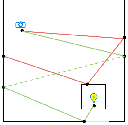
With unidirectional path tracing, rays are cast starting at the camera and bounce around the scene. At each bounce, a "shadow ray" is cast directly to the light to measure direct lighting. In the situation depicted in Figure X, a vertex will rarely be sampled in the region illuminated by the light prior to casting a shadow ray. However, with bidirectional path tracing (BDPT), two independent paths are traced: one starting at the camera, and one starting at the light. Then, each subpath is connected resulting in a complete path from light to camera. It is not always possible to connect the subpaths, but this strategy is generally more successful at sampling paths. If many paths have no or little contribution, yet some have high contribution, this will result in variance.

With BDPT, light subpath \(q_0,\dots,q_{s-1}\) consisting of \(s\) vertices is constructed incrementally, starting with a point \(q_0\) on a light, and a camera subpath \(p_0,\dots,p_{t-1}\) is constructed incrementally, starting with a point \(p_0\) on the camera, resulting in a composite path proceeding from the light to the camera:

\[\bar{p} = q_0,\dots,q_{s-1},p_0,\dots,p_{t-1}.\]

The specification \((s,t)\) of the number of light and camera vertices is called a strategy or a technique. For strategies with \(t \ge 2\), at the point \(p_0\) (which, on a pinhole camera is a fixed point), a direction is sampled which proceeds from this point through the image plane, thus designating a particular pixel. The next vertex \(p_1\) is found by computing the closest intersection along this direction, if any. Likewise, a point \(q_0\) is sampled on the light and then a direction is sampled and an intersection is performed to compute the next vertex \(q_1\), etc. Finally, a connection is performed between vertices \(p_{t-1}\) and \(q_{s-1}\); these vertices are connectable if they are mutually visible (a ray can be cast between them without being occluded). However, the path throughput might be \(0\) if the BSDFs at the vertices do not scatter light in the respective direction (e.g. a connection containing a vertex on a perfect specular surface is unlikely to succeed since it is unlikely that the connection coincides with the reflection direction).

BDPT implementations typically involve a few techniques used to improve its efficiency. First, prefixes of the light and camera subpaths, once generated, are reused, as in Figure 24.

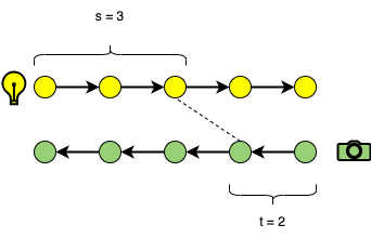
Note, however, that in the Multiplexed Metropolis Light Transport algorithm, subpaths are not reused in this manner; instead, a single strategy is selected using Metropolis sampling.

The second technique used to improve the efficiency of BDPT is multiple importance sampling. Multiple importance sampling (MIS) is used to compute a probability density function (PDF) for path construction. The balance heuristic is used to weight path contributions. In order to employ this heuristic, the probability densities for all hypothetical path constructions must be known. Figure 25 depicts an actual strategy and all other hypothetical strategies.

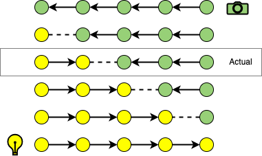
We can denote a path \(\bar{x}\) of length \(n\) constructed with strategy \((s,t)\) (where \(s + t = n\)), from camera subpath \(p_o,\dots,p_{t-1}\) and light subpath \(q_0,\dots,q_{s-1}\) as

\[\bar{x} = x_0,\dots,x_{n-1} = q_0,\dots,q_{s-1},p_0,\dots,p_{t-1}.\]

Each vertex is denoted \(x_i\) for \(0 \leq i \lt n\). Note that the PDFs for vertices are computed with respect to area (they are PDFs per unit area). The expression \(p^{\rightarrow}(x_i)\) represents the PDF per unit area of sampling vertex \(x_i\) along a light subpath. The expression \(p^{\leftarrow}(x_i)\) represents the PDF per unit area of sampling vertex \(x_i\) along a camera subpath. These will generally differ since they will involve conversions from solid angle densities of different BRDFs, etc. The path density for the actual strategy \((s,t)\) is denoted \(p_s(\bar{x})\) (where implicitly \(t = n - s\)) and is given by

\begin{align}p_s(\bar{x}) &= p^{\rightarrow}(q_0),\dots,p^{\rightarrow}(q_{s-1}),p^{\leftarrow}(p_{t-1}),\dots,p^{\leftarrow}(p_0) \\&= p^{\rightarrow}(x_0),\dots,p^{\rightarrow}(x_{s-1}),p^{\leftarrow}(x_s),\dots,p^{\leftarrow}(x_{n-1}).\end{align}

For a given actual strategy \((s,t)\) used to construct a given path, we want to consider each hypothetical strategy \((i,j)\) which could have been used to construct the same path. Thus, it must be the case that \(i+j = s+t\) in order to preserve path length. We denote the path density of a hypothetical path construction with strategy \((i,j)\) on path \(\bar{x}\) as \(p_i(\bar{x})\), where implicitly \(j = n - i\):

\[p_i(\bar{x}) = p^{\rightarrow}(x_0),\dots,p^{\rightarrow}(x_{i-1}),p^{\leftarrow}(x_i),\dots,p^{\leftarrow}(x_{n-1}).\]

To compute the MIS weight \(w_s(\bar{x})\) for an actual strategy \(s\), we must compute

\[w_s = \frac{p(\bar{x})}{\sum_{i=1}^np_i(\bar{x})}.\]

There is an efficient and more numerically stable way to compute the MIS weight which I learned from PBRT.

First, divide both numerator and denominator of \(w_s(\bar{x})\) by \(p_s(\bar{x})\) to obtain the equivalent expression

\[w_s = \frac{1}{\sum_{i=1}^n\frac{p_i(\bar{x})}{p_s(\bar{x})}}.\]

Next, split this expression as follows (noting that \(p_i(\bar{x}) = p_s(\bar{x}\) when \(i = s\)):

\[w_s = \left(\sum_{i=1}^{s-1}\frac{p_i(\bar{x})}{p_s(\bar{x})} + 1 + \sum_{i=s+1}^{n}\frac{p_i(\bar{x})}{p_s(\bar{x})} \right)^{-1}.\]

Denote the ratios therein as follows:

\[r_i(\bar{x}) = \frac{p_i(\bar{x})}{p_s(\bar{x})}.\]

These ratios can be defined recursively as follows:

\[r_i(\bar{x}) = \begin{cases}\frac{p_i(\bar{x})}{p_{i+1}(\bar{x})}\frac{p_{i+1}(\bar{x})}{p_s(\bar{x})} = \frac{p_i(\bar{x})}{p_{i+1}(\bar{x})}r_{i+1}(\bar{x}) & (i \lt s), \\ 1 & (i = s), \\ \frac{p_i(\bar{x})}{p_{i-1}(\bar{x})}\frac{p_{i-1}(\bar{x})}{p_s(\bar{x})} = \frac{p_i(\bar{x})}{p_{i-1}(\bar{x})}r_{i-1}(\bar{x}) & (i \gt s).\end{cases}\]

The ratios between path densities of strategies that differ by \(1\) share all terms except for one:

\[\frac{p_i(\bar{x})}{p_{i-1}(\bar{x})} = \frac{p^{\rightarrow}(x_0)\dots p^{\rightarrow}(x_{i-1})p^{\leftarrow}(x_i)p^{\leftarrow}(x_{i+1})\dots p^{\leftarrow}(x_{n-1})}{p^{\rightarrow}(x_0)\dots p^{\rightarrow}(x_{i-1})p^{\rightarrow}(x_i)p^{\leftarrow}(x_{i+1})\dots p^{\leftarrow}(x_{n-1})} = \frac{p^{\leftarrow}(x_i)}{p^{\rightarrow}(x_i)},\]

\[\frac{p_i(\bar{x})}{p_{i-1}(\bar{x})} = \frac{p^{\rightarrow}(x_0)\dots p^{\rightarrow}(x_{i-2})p^{\rightarrow}(x_{i-1})p^{\leftarrow}(x_i) \dots p^{\leftarrow}(x_{n-1})}{p^{\rightarrow}(x_0)\dots p^{\rightarrow}(x_{i-2})p^{\leftarrow}(x_{i-1})p^{\leftarrow}(x_i) \dots p^{\leftarrow}(x_{n-1})} = \frac{p_{\rightarrow}(x_{i-1})}{p^{\rightarrow}(x_{i-1})}.\]

Thus, we can rewrite the recurrence relation as

\[r_i(\bar{x}) = \begin{cases}\frac{p_i(\bar{x})}{p_{i+1}(\bar{x})}\frac{p_{i+1}(\bar{x})}{p_s(\bar{x})} = \frac{p^{\leftarrow}(x_i)}{p^{\rightarrow}(x_i)}r_{i+1}(\bar{x}) & (i \lt s), \\ 1 & (i = s), \\ \frac{p_i(\bar{x})}{p_{i-1}(\bar{x})}\frac{p_{i-1}(\bar{x})}{p_s(\bar{x})} = \frac{p^{\rightarrow}(x_{i-1})}{p^{\rightarrow}(x_{i-1})}r_{i-1}(\bar{x}) & (i \gt s).\end{cases}\]

Finally, another technique used to improve the efficiency of BDPT is specialized sampling from cameras and lights; strategies where \(s=1\) or \(t=1\) are unlikely to succeed without specialized sampling.

Metropolis Light Transport

Researchers Veach and Guibas [3] proposed the Metropolis Light Transport (MLT) algorithm which combines bidirectional path tracing with Metropolis sampling.

Let us write the measurement equation for pixel \(j\) as

\[I_j = \int_{\Omega}h_j(\bar{x})f(\bar{x})d\mu(\bar{x}).\]

To apply Metropolis sampling to compute this integral, we need to define the acceptance probability, which is a scalar function. However, in rendering, the functions used are spectral distributions. We designate a scalar contribution function \(I(\bar{x})\) which is proportional to the spectral radiance.

In practice, we choose luminance, which is spectral radiance integrated against a particular spectral response function \(V(\lambda)\):

\[Y = \int L_{\lambda}(\lambda)V(\lambda)~d\lambda.\]

Thus, we choose \(I = Y\). Then, the distribution corresponding to \(I(\bar{x})\) is

\[p(\bar{x}) = \frac{I(\bar{x})}{\int_{\Omega} I(\bar{x})~d\mu(\bar{x})}.\]

Then, we can apply Metropolis sampling to generate samples proportional to this distribution. The Monte Carlo estimator will be

\begin{align}I_j &\approx \frac{1}{n}\sum_{i=1}^n \frac{h_j(\bar{x}_i)f(\bar{x}_i)}{p(\bar{x}_i)} \\&= \frac{1}{n}\sum_{i=1}^n \frac{h_j(\bar{x}_i)f(\bar{x}_i)}{\frac{I(\bar{x})}{\int_{\Omega} I(\bar{x})~d\mu(\bar{x})}} \\&= \frac{1}{n}\sum_{i=1}^n \frac{h_j(\bar{x}_i)f(\bar{x}_i)}{I(\bar{x}_i)}\left(\int_{\Omega} I(\bar{x})~d\mu(\bar{x})\right).\end{align}

Using the notation

\[b = \int_{\Omega} I(\bar{x})~d\mu(\bar{x}),\]

we then obtain

\[I_j = \frac{b}{n}\sum_{i=1}^n \frac{h_j(\bar{x}_i)f(\bar{x}_i)}{I(\bar{x}_i)}\].

In practice, an initialization phase computes the value \(b\) for some fixed number of samples, and then it is used when calculating each integral \(I_j\).

The original MLT algorithm involved computing various path mutations, and the algorithm is intricate and fairly difficult to implement. Therefore Kelemen, et. al [2] proposed a variant called Primary Sample Space Metropolis Light Transport (PSSMLT) which mutates paths in the primary sample space, which is simply the space of vectors of uniformly-distributed random numbers used to generate samples (ultimately, all samples are based on such numbers drawn from PRNGs). Thus, each path is simply a tuple of numbers, each in the range \([0,1]\). Such samples are easy to manipulate (e.g. by adding small perturbations to each sample). Furthermore, this approach permits Metropolis sampling to be used to generate samples for any algorithm (whether path tracing, or BDPT, etc.), since such algorithms use samples drawn from uniform distributions.

We must re-express the contribution function in the primary sample space. Let \(S(\bar{x})\) denote the mapping from the primary sample space to the path space. Then, the formula for the pullback of top-level differential forms (integrands here) indicates that

\[F^*(u dy^1 \wedge \dots \wedge dy^n) = (u \circ F)(\mathrm{det DF})dx^1 \wedge \dots \wedge dx^n,\]

where \(DF\) is the Jacobian matrix of the smooth map \(F\).

In the context of the contribution function, when pulling back along the map \(S\), this yields

\begin{align}\int_{\Omega}I(\bar{x})~d\mu(\bar{x}) &= \int_{\mathcal{U}}S^*\left(I(\bar{x})~d\mu(\bar{x})\right) \\&= \int_{\mathcal{U}}I(S(\bar{y})) (\mathrm{det} DS)d\mu(\bar{y}).\end{align}

Thus, we work with a new scalar contribution function \(I^*\) defined so that

\[I^*(\bar{y}) = I(S(\bar{y})) (\mathrm{det} DS).\]

However, we do not actually need to compute the Jacobian determinant \(\mathrm{det} DS\) directly. The same transformation applies to probability distribution functions, so we can relate the distributions as follows:

\[p^*(\bar{y}) = p(S(\bar{y}))(\mathrm{det} DS).\]

However, the PDF for sampling an \(n\)-dimensional uniform random variable on the unit hypercube \([0,1]^n\) is a constant \(1\), i.e. \(p^*(\bar{y}) = 1\). Thus, we can rewrite the previous equation as

\[(\mathrm{det} DS) = \frac{1}{p(S(\bar{y}))}.\]

This means that

\[I^*(\bar{y}) = \frac{I(S(\bar{y}))}{p(S(\bar{y}))}.\]

In the primary sample space, the transition probabilities are symmetric, and thus the acceptance probability becomes:

\[a(\bar{u}_i \rightarrow \bar{v}) = \frac{I^*(\bar{v})}{I^*(\bar{u}_i)}.\]

The PSSMLT algorithm proposes two types of primary sample space mutations. The first is a small step mutation which introduces small perturbations to each element of the sample vectors of random numbers; this can be performed, for instance, by sampling and offset from a normal (Gaussian) distribution with a given standard deviation \(\sigma\) and adding the offset to the current value. The second type of mutation is a large step mutation, which replaces the entire sample with newly generated uniformly distributed random variables.

These two sampling technique are then combined using multiple importance sampling (in particular, the balance heuristic). Metropolis sampling generates samples in proportion to the scalar contribution function's density, which is

\[p_1(\bar{x}) = \frac{I^*(\bar{x})}{b}.\]

The large step sampling generates uniformly distributed samples, so its density is constant, i.e.

\[p_2(\bar{x}) = 1.\]

Combining these with the balance heuristic yields

\[w(\bar{u}) = \frac{1}{m_1p_1(\bar{u}) + m_2p_2(\bar{u}}),\]

where \(m_i\) is the number of samples generated by each. However, if the probability of choosing the large step is \(p_{\text{large}}\), then we can set \(m = m_1\) and \(m_2 = p_{\text{large}}m\).

Mean value substitution is used, so the contribution of a prior Metropolis sample should be

\[(1 - a) \cdot w(\bar{u}) \cdot f^*(\bar{u}) = \frac{(1 - a) \cdot f^*(\bar{u})}{\left(\frac{I^*(\bar{u})}{b} + p_{\text{large}}\right)m}.\]

For large steps, the contribution is made by both Metropolis sampling and the uncorrelated method, so the weighted contribution is

\[a \cdot w(\bar{u}) \cdot f^*(\bar{u}) + w(\bar{u}) \cdot f^*(\bar{u}) = \frac{(a + 1) \cdot f^*(\bar{u})}{\left(\frac{I^*(\bar{u})}{b} + p_{\text{large}}\right)m}.\]

Small steps originate from Metropolis sampling alone. Thus, their weighted contribution is

\[a \cdot w(\bar{u}) \cdot f^*(\bar{u})= \frac{a \cdot f^*(\bar{u})}{\left(\frac{I^*(\bar{u})}{b} + p_{\text{large}}\right)m}.\]

The two weights for proposal contributions can be combined as

\[\frac{(a + L) \cdot f^*(\bar{u})}{\left(\frac{I^*(\bar{u})}{b} + p_{\text{large}}\right)m},\]

where \(L = 1\) in the case of a large step, and \(0\) in the case of a small step.

The Multiplexed Metropolis Light Transport (MMLT) algorithm by Hachisuka, et. al. [1] introduces a variant to PSSMLT. In this variant, the BDPT connection strategy is added as an additional state in a Markov chain. Then, \(N\) independent Markov chains are used, one for each path length. After calculating the integrals for each scalar contribution function, one for each path length, a PDF is constructed. This PDF is then used to sample a random path length in a manner proportional to its contribution.

Materials and Textures

A texture maps points on a surface to various data (for instance colors). A constant texture is the simplest texture, which, for instance, computes the same color for every point on a surface. An image texture could map an image onto a surface, thus computing a different color for each point on the surface. A material combines one or more textures with a BSDF and initializes the parameters of the BSDF with data computed from the textures.

Imaging

After integration is complete, the result is an array of radiant power estimates, one per pixel. Depending on the implementation, this is either directly computed in a linear color space, or it is computed as a set of spectral distributions which are then converted to a linear color space, etc. In order to display this as an image, several adjustments must be made.

Gamma Correction

Human perception of brightness is non-linear. Compute monitors will adjust for this by scaling tristimulus values (e.g. RGB) according to a power function:

\[v_o = v_i^{\gamma},\]

where gamma is \(2.2\) for many monitors.

In order to compensate for this, gamma correction scales the resulting tristimulus values \(v_r\) by the reciprocal, such that

\[v_o = v_i^{\gamma} = (v_r^{\frac{1}{\gamma}})^{\gamma} = v_r.\]

Tone Mapping

Additionally, the radiant power computed does not match the dynamic range required by most image formats. The process of tone mapping rescales the values to a desired range. For instance, to rescale on the range of \([0,255]\), the following simple tone mapping can be applied:

\[v_o = (1 - e^{-v_i}) \cdot 255\]

Supersampling

Supersampling is a technique for creating an image that is larger than necessary and downscaling it (using a suitable filter function to combine multiple pixels into one) to produce a higher quality image.

Future Work

The prototype implementation described in this post could be extended to a more fully-featured renderer by including the following features:

• Support for rendering volumes (also called participating media) in order to represent scattering that occurs inside surfaces. This can be used to represent wax, skin, fog, clouds, smoke, liquids, etc.
• Support for spectral rendering, as described briefly in this post.
• Support for additional geometry, including triangle meshes and curves, and techniques such as instancing.
• Support for acceleration structures, in particular bounding volume hierarchies.
• Support for textures (i.e. image textures, etc.)
• Support for error bounding (i.e. systematically tracking the upper bounds on floating point operations in order to perform ray intersection tests more accurately). This also includes techniques such as ray differentials used for texture mapping, etc.
• Support for normal maps, bump maps, etc. which allow perturbations of the geometric normals in order to simulate more complex object appearances without introducing additional geometric overhead.
• Support for local coordinates (transformations)
• Support for additional camera models, such as orthographic cameras and various lens models.
• Support for additional rendering algorithms, such as unidirectional path tracing, bidirectional path tracing (without Metropolis Sampling, and with minor variants in path construction), etc.
• Support for additional sampling algorithms
• Support for additional light types, such as point lights, infinite area lights, directional (spot) lights, etc. and emissive materials.
• Support for GPU rendering and accelerated CPU rendering (using SIMD and multithreading).

With a feature set such as the one described above, a renderer could, in principle, render many models published on popular websites by artists.

Further Reading

The single most useful resource that I found was the book Physically Based Rendering: From Theory to Implementation. The third edition contains information about bidirectional path tracing and Metropolis Light Transport. The fourth edition is the latest edition as of the writing of this post. Both the third and fourth editions are freely available online. As the title implies, this book contains comprehensive descriptions of both the theory and practice of physically-based rendering. Additionally, the source code for the pbrt renderer is available on GitHub here.

References

• [1] The paper on the MMLT algorithm: Multiplexed Metropolis Light Transport. Toshiya Hachisuka, Anton S. Kaplanyan, and Carsten Dachsbacher. 2014. Multiplexed metropolis light transport. ACM Trans. Graph. 33, 4, Article 100 (July 2014), 10 pages. https://doi.org/10.1145/2601097.2601138
• [2] The paper on the PSSMLT algorithm: Primary Sample Space Metropolis Light Transport. Kelemen, Csaba & Szirmay-Kalos, László & Antal, Gyorgy & Csonka, Ferenc. (2002). A Simple and Robust Mutation Strategy for the Metropolis Light Transport Algorithm. Comput. Graph. Forum. 21. 10.1111/1467-8659.t01-1-00703
• [3] The paper on the original MLT algorithm: Metropolis Light Transport. Eric Veach and Leonidas J. Guibas. 1997. Metropolis light transport. In Proceedings of the 24th annual conference on Computer graphics and interactive techniques (SIGGRAPH '97). ACM Press/Addison-Wesley Publishing Co., USA, 65–76. https://doi.org/10.1145/258734.258775
• Eric Veach's PhD thesis
• The Physically Based Rendering Book